arrow-left

All pages
gitbookPowered by GitBook
1 of 6

Loading...

Loading...

Loading...

Loading...

Loading...

Loading...

DS-Explained-Simple

hashtag
Linear Data Structures

Linear data structures store elements in a sequential manner. These are the most fundamental and widely used data structures.

  • Array/List – An array or list is a linear data structure where elements are stored in a sequential manner, numbered from 0 to n-1, where n is the size of the array. The array elements can be accessed using their index.

  • Stacks – A stack is a linear data structure that stores data in a Last In, First Out (LIFO) manner.

  • Queues – A data structure that stores data in a First In, First Out (FIFO) manner.

  • Linked Lists – A linear data structure that stores elements sequentially but cannot be accessed directly using an index. It consists of links to the next item, along with the data.

hashtag
Non-Linear Data Structures

Non-Linear data structures are more complex data structures, that are not sequential in manner.

  • Trees – Trees store data in a tree-like manner. They consist of a root, which contains the data and links to children nodes. The children nodes may in turn contain more children. They are the building blocks of many other Data Structures.

  • Heaps – A heap is a tree, which is used as a priority queue. There are max-heaps, and min-heaps that contain the maximum value and the minimum value at the root node, respectively.

  • Hash Tables – Hash Tables are data structures that contain key-value pairs. They use the concept of hashing to determine the keys in the tables. Usually used for quick access of values.

hashtag
Python Collections and In-Built Data Structures

  • Tuples – They are sequential data structures, that are similar to lists, but they’re immutable.

  • Dictionary – Dictionaries are python-specific data structures that are similar to hashtables, and are used for quick access of values.

  • Sets – A collection of unordered distinct elements, that have quick access time.

Now that we have an overview of data structures, let’s delve into the nuances of each of them in the upcoming articles of the series. Here are some resources to get you started with interview and programming preparation.

hashtag
Choose a Platform

There are numerous platforms like , , , , , , , , etc. to learn programming. Out of these, after a lot of trial and error I felt that a combination of HackerRank and LeetCode worked really well for preparing for interviews.

HackerRank

HackerRank is amazing because it has customized tracks for each programming language, and one each for data structures and algorithms. There are also customized filters for each DS type like Stack, Queue, etc.

LeetCode

LeetCode is an excellent website for company-specific preparation. If you pay for LeetCode Premium, you get company-specific questions. This is great for preparing for companies like FaceBook, Microsoft, NetFlix, Amazon, Apple, Google, etc. They also have contests and real-time mock interviews that boost your confidence and skills.

hashtag
Implement the Data Structures from Scratch

By personal experience, implementing the data structures from scratch helps a lot. It helps you to understand the data structure in detail and helps in debugging, in case you run into any errors. Python offers in-build implementation for many data structures, but it is better to learn how to implement it at least once.

  • Graphs – Graphs are complex data structures that implement a collection of nodes, connected together by vertices.

  • Collections – Collections are a group of optimized implementations for data structures like dictionaries, maps, tuples, queues.

    LeetCodearrow-up-right
    HackerRankarrow-up-right
    InterviewBitarrow-up-right
    TopCoderarrow-up-right
    HackerEartharrow-up-right
    CodeChefarrow-up-right
    CodeForcesarrow-up-right
    SPOJarrow-up-right

    General Data Structures Notes

    Data Typesarrow-up-right

    • Data Structuresarrow-up-right

    • Arrayarrow-up-right

    In this post we will be looking briefly at, and at a high-level, the various data types and data structures used in designing software systems, and from which specific types of algorithms can subsequently be built upon and optimized for.

    There are many data structures, and even the ones that are covered here have many nuances that make it impossible to cover every possible detail. But my hope is that this will give you an interest to research them further.

    But before we get into it... time for some self-promotion 🙊

    hashtag
    Data Types

    A data type is an of data which tells the compiler (or interpreter) how the programmer intends to use the data.

    • Scalar: basic building block (boolean, integer, float, char etc.)

    • Composite: any data type (struct, array, string etc.) composed of scalars or composite types (also referred to as a ‘compound’ type).

    • Abstract: data type that is defined by its behaviour (tuple, set, stack, queue, graph etc).

    NOTE: You might also have heard of a ‘primitive’ type, which is sometimes confused with the ‘scalar’ type. A primitive is typically used to represent a ‘value type’ (e.g. pass-by-value semantics) and this contrasts with ‘reference types’ (e.g. pass-by-reference semantics).

    If we consider a composite type, such as a ‘string’, it describes a data structure which contains a sequence of char scalars (characters), and as such is referred to as being a ‘composite’ type. Whereas the underlying implementation of the string composite type is typically implemented using an array data structure (we’ll cover shortly).

    Note: in a language like C the length of the string’s underlying array will be the number of characters in the string followed by a ‘’.

    An abstract data type (ADT) describes the expected behaviour associated with a concrete data structure. For example, a ‘list’ is an abstract data type which represents a countable number of ordered values, but again the implementation of such a data type could be implemented using a variety of different data structures, one being a ‘’.

    Note: an ADT describes behaviour from the perspective of a consumer of that type (e.g. it describes certain operations that can be performed on the data itself). For example, a list data type can be considered a sequence of values and so one available operation/behaviour would be that it must be iterable.

    hashtag
    Data Structures

    A data structure is a collection of data type ‘values’ which are stored and organized in such a way that it allows for efficient access and modification. In some cases a data structure can become the underlying implementation for a particular data type.

    For example, composite data types are data structures that are composed of scalar data types and/or other composite types, whereas an abstract data type will define a set of behaviours (almost like an ‘interface’ in a sense) for which a particular data structure can be used as the concrete implementation for that data type.

    When we think of data structures, there are generally four forms:

    1. Linear: arrays, lists

    2. Tree: binary, heaps, space partitioning etc.

    3. Hash: distributed hash table, hash tree etc.

    Note: for a more complete reference, please see this .

    Let’s now take a look at the properties that make up a few of the more well known data structures.

    hashtag
    Array

    An array is a finite group of data, which is allocated contiguous (i.e. sharing a common border) memory locations, and each element within the array is accessed via an index key (typically numerical, and zero based).

    The name assigned to an array is typically a pointer to the first item in the array. Meaning that given an array identifier of arr which was assigned the value ["a", "b", "c"], in order to access the "b" element you would use the index 1 to lookup the value: arr[1].

    Arrays are traditionally ‘finite’ in size, meaning you define their length/size (i.e. memory capacity) up front, but there is a concept known as ‘dynamic arrays’ (and of which you’re likely more familiar with when dealing with certain high-level programmings languages) which supports the growing (or resizing) of an array to allow for more elements to be added to it.

    In order to resize an array you first need to allocate a new slot of memory (in order to copy the original array element values over to), and because this type of operation is quite ‘expensive’ (in terms of computation and performance) you need to be sure you increase the memory capacity just the right amount (typically double the original size) to allow for more elements to be added at a later time without causing the CPU to have to resize the array over and over again unnecessarily.

    One consideration that needs to be given is that you don’t want the resized memory space to be too large, otherwise finding an appropriate slot of memory becomes more tricky.

    When dealing with modifying arrays you also need to be careful because this requires significant overhead due to the way arrays are allocated memory slots.

    So if you imagine you have an array and you want to remove an element from the middle of the array, try to think about that in terms of memory allocation: an array needs its indexes to be contiguous, and so we have to re-allocate a new chunk of memory and copy over the elements that were placed around the deleted element.

    These types of operations, when done at scale, are the foundation behind why it’s important to have an understanding of how data structures are implemented. The reason being, when you’re writing an algorithm you will hopefully be able to recognize when you’re about to do something (let’s say modify an array many times within a loop construct) that could ultimately end up being quite a memory intensive set of operations.

    Note: interestingly I’ve discovered that in some languages an array (as in the composite data type) has been implemented using a variety of different data structures such as hash table, linked list, and even a search tree.

    hashtag
    Linked List

    A linked list is different to an array in that the order of the elements within the list are not determined by a contiguous memory allocation. Instead the elements of the linked list can be sporadically placed in memory due to its design, which is that each element of the list (also referred to as a ‘node’) consists of two parts:

    1. the data

    2. a pointer

    The data is what you’ve assigned to that element/node, whereas the pointer is a memory address reference to the next node in the list.

    Also unlike an array, there is no index access. So in order to locate a specific piece of data you’ll need to traverse the entire list until you find the data you’re looking for.

    This is one of the key performance characteristics of a linked list, and is why (for most implementations of this data structure) you’re not able to append data to the list (because if you think about the performance of such an operation it would require you to traverse the entire list to find the end/last node). Instead linked lists generally will only allow prepending to a list as it’s much quicker. The newly added node will then have its pointer set to the original ‘head’ of the list.

    There is also a modified version of this data structure referred to as a ‘doubly linked list’ which is essentially the same concept but with the exception of a third attribute for each node: a pointer to the previous node (whereas a normal linked list would only have a pointer to the following node).

    Note: again, performance considerations need to be given for the types of operations being made with a doubly linked list, such as the addition or removal of nodes in the list, because you now have not only the pointers to the following node that need to be updated, but also the pointers back to a previous node that now also need to be updated.

    hashtag
    Tree

    The concept of a ‘tree’ in its simplest terms is to represent a hierarchical tree structure, with a root value and subtrees of children (with a parent node), represented as a set of linked nodes.

    A tree contains “nodes” (a node has a value associated with it) and each node is connected by a line called an “edge”. These lines represent the relationship between the nodes.

    The top level node is known as the “root” and a node with no children is a “leaf”. If a node is connected to other nodes, then the preceeding node is referred to as the “parent”, and nodes following it are “child” nodes.

    There are various incarnations of the basic tree structure, each with their own unique characteristics and performance considerations:

    • Binary Tree

    • Binary Search Tree

    • Red-Black Tree

    hashtag
    Binary Tree

    A binary tree is a ‘rooted tree’ and consists of nodes which have, at most, two children. This is as the name suggests (i.e. ‘binary’: 0 or 1), so two potential values/directions.

    Rooted trees suggest a notion of distance (i.e. distance from the ‘root’ node)

    Note: in some cases you might refer to a binary tree as an ‘undirected’ graph (we’ll look at shortly) if talking in the context of graph theory or mathematics.

    Binary trees are the building blocks of other tree data structures (see also: for more details), and so when it comes to the performance of certain operations (insertion, deletion etc) consideration needs to be given to the number of ‘hops’ that need to be made as well as the re-balancing of the tree (much the same way as the pointers for a linked list need to be updated).

    hashtag
    Binary Search Tree

    A binary search tree is a ‘sorted’ tree, and is named as such because it helps to support the use of a ‘binary search’ algorithm for searching more efficiently for a particular node (more on that later).

    To understand the idea of the nodes being ‘sorted’ (or ‘ordered’) we need to compare the left node with the right node. The left node should always be a lesser number than the right node, and the parent node should be the decider as to whether a child node is placed to the left or the right.

    Consider the example image above, where we can see the root node is 8. Let’s imagine we’re going to construct this tree.

    We start with 8 as the root node and then we’re given the number 3 to insert into the tree. At this point the underlying logic for constructing the tree will know that the number 3 is less than 8 and so it’ll first check to see if there is already a left node (there isn’t), so in this scenario the logic will determine that the tree should have a new left node under 8 and assign it the value of 3.

    Now if we give the number 6 to be inserted, the logic will find that again it is less than 8 and so it’ll check for a left node. There is a left node (it has a value of 3) and so the value 6 is greater than 3. This means the logic will now check to see if there is a right node (there isn’t) and subsequently creates a new right node and assigns it the value 6.

    This process continues on and on until the tree has been provided all of the relevant numbers to be sorted.

    In essence what this sorted tree design facilitates is the means for an operation (such as lookup, insertion, deletion) to only take, on average, time proportional to the of the number of items stored in the tree.

    So if there were 1000 nodes in the tree, and we wanted to find a specific node, then the average case number of comparisons (i.e. comparing left/right nodes) would be 10.

    By using the logarithm to calculate this we get: log 2(10) = 1024 which is the inverse of the exponentiation 2^10 (“2 raised to the power of 10”), so this says we’ll execute 10 comparisons before finding the node we were after.

    To break that down a bit further: the exponentiation calculation is 1024 = 2 × 2 × 2 x 2 x 2 x 2 × 2 × 2 x 2 x 2 = 2^10, so the “logarithm to base 2” of 10 is 1024.

    The logarithm (i.e. the inverse function of exponentiation) of 1000 to base 2, in this case abstracted to n, is denoted as log 2 (n), but typically the base 2 is omitted to just log(n).

    When determining the ‘time complexity’ for operations on this type of data structure we typically use ‘Big O’ notation and thus the Big O complexity would be defined as O(log n) for the average search case (which is good), but the worst case for searching would still be O(n) linear time (which is bad – and I’ll explain why in the next section on ).

    Note: I’ve covered the basics of logarithm and binary search in a about Big O notation, and so I’ll refer you to that for more details.

    Similarly when considering complexity for a particular algorithm, we should take into account both ‘time’ and ‘space’ complexity. The latter is the amount of memory necessary for the algorithm to execute and is similar to time complexity in that we’re interested in how that resource (time vs space) will change and affect the performance depending on the size of the input.

    hashtag
    Red-Black Tree

    The performance of a binary search tree is dependant on the height of the tree. Meaning we should aim to keep the tree as ‘balanced’ as possible, otherwise the logarithm performance is lost in favor of linear time.

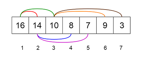
    To understand why that is, consider the following data stored in an array:

    If we construct a binary search tree from this data, what we would ultimately end up with is a very ‘unbalanced’ tree in the sense that all the nodes would be to the right, and none to the left.

    When we search this type of tree (which for all purposes is effectively a linked list) we would, worst case, end up with linear time complexity: O(n). To resolve that problem we need a way to balance the nodes in the tree.

    This is where the concept of a red-black tree comes in to help us. With a red-black tree (due to it being consistently balanced) we get O(log n) for search/insert/delete operations (which is great).

    Let’s consider the properties of a red-black tree:

    • Each node is either red or black.

    • The root node is always black.

    • All leaves are ‘NIL’ and should also be black.

    Note: when counting nodes we don’t include the root node, and we count each black node up to (and including) the NIL node.

    The height of the tree is referred to as its ‘black-height’, which is the number of black nodes (not including the root) to the furthest leaf, and should be no longer than twice as long as the length of the shortest path (the nearest NIL).

    These properties are what enable the red-black tree to provide the performance characteristics it has (i.e. O(log n)), and so whenever changes are made to the tree we want to aim to keep the tree height as short as possible.

    On every node insertion, or deletion, we need to ensure we have not violated the red-black properties. If we do, then there are two possible steps that we have to consider in order to keep the tree appropriately balanced (which we’ll check in this order):

    1. Recolour the node in the case of a red node no longer having two black child nodes.

    2. Make a (left/right) in the case where recolouring then requires a structural change.

    The goal of a rotation is to decrease the height of the tree. The way we do this is by moving larger subtrees up the tree, and smaller subtrees down the tree. We rotate in the direction of the smaller subtree, so if the smaller side is the right side we’ll do a right rotation.

    Note: there is an inconsistency between what node/subtree is affected by a rotation. Does the subtree being moved into the parent position indicate the direction or does the target node affected by the newly moved subtree indicate the direction (I’ve opted for the latter, as we’ll see below, but be aware of this when reading research material).

    In essence there are three steps that need to be applied to the target node (T) being rotated, and this is the same for either a left rotation or a right rotation. Let’s quickly look at both of these rotation movements:

    • Left Rotation:

      1. T’s right node (R) is unset & becomes T’s parent †

    † we now find R’s left pointer has to be set to T (in order for it to become the parent node), meaning R’s original left pointer is orphaned.

    • Right Rotation:

      1. T’s left node (L) is unset & becomes T’s parent †

    † we now find L’s right pointer has to be set to T (in order for it to become the parent node), meaning L’s original right pointer is orphaned.

    Let’s now visualize the movements for both rotations:

    Left Rotation

    Right Rotation

    Note: rotations are confusing, so I recommend watching for some examples and pseudo-code.

    hashtag
    B-tree

    A B-tree is a sorted tree that is very similar in essence to a red-black tree in that it is self-balancing and as such can guarantee logarithmic time for search/insert/delete operations.

    A B-tree is useful for large read/writes of data and is commonly used in the design of databases and file systems, but it’s important to note that a B-tree is not a binary search tree because it allows more than two child nodes.

    The reasoning for allowing multiple children for a node is to ensure the height of the tree is kept as small as possible. The rationale is that B-trees are designed for handling huge amounts of data which itself cannot exist in-memory, and so that data is pulled (in chunks) from external sources.

    This type of I/O is expensive and so keeping the tree ‘fat’ (i.e. to have a very short height instead of lots of node subtrees creating extra length) helps to reduce the amount of disk access.

    The design of a B-tree means that all nodes allow a set range for its children but not all nodes will need the full range, meaning that there is a potential for wasted space.

    Note: there are also variants of the B-tree, such as B+ trees and B* trees (which we’ll leave as a research exercise for the reader).

    hashtag
    Weight-balanced Tree

    A weight-balanced tree is a form of binary search tree and is similar in spirit to a weighted graph, in that individual nodes are ‘weighted’ to indicate the more likely successful route with regards to searching for a particular value.

    The search performance is the driving motivation for using this data structure, and typically used for implementing sets and dynamic dictionaries.

    hashtag
    Binary Heap

    A binary heap tree is a binary tree, not a binary search tree, and so it’s not a sorted tree. It has some additional properties that we’ll look at in a moment, but in essence the purpose of this data structure is primarily to be used as the underlying implementation for a .

    The additional properties associated with a binary heap are:

    • heap property: the node value is either greater (or lesser depending on the direction of the heap) or equal to the value of its parent.

    • shape property: if the last level of the tree is incomplete, the missing nodes are filled.

    The insertion and deletion operations yield a time complexity of O(log n).

    Below are some examples of a max and min binary heap tree structure.

    Max Heap:

    Min Heap:

    hashtag
    Hash Table

    A hash table is a data structure which is capable of maping ‘keys’ to ‘values’, and you’ll typically find this is abstracted and enhanced with additional behaviours by many high-level programming languages such that they behave like an ‘’ abstract data type.

    In Python it’s called a ‘dictionary’ and has the following structure (on top of which are functions such as del, get and pop etc that can manipulate the underlying data):

    The keys for the hash table are determined by way of a but implementors need to be mindful of hash ‘collisions’ which can occur if the hash function isn’t able to create a distinct or unique key for the table.

    The better the hash generation, the more distributed the keys will be, and thus less likely to collide. Also the size of the underlying array data structure needs to accommodate the type of hash function used for the key generation.

    For example, if using modular arithmetic you might find the array needs to be sized to a prime number.

    There are many techniques for resolving hashing collisions, but here are two that I’ve encountered:

    1. Separate Chaining

    2. Linear Probing

    hashtag
    Separate Chaining

    With this option our keys will contain a nested data structure, and we’ll use a technique for storing our conflicting values into this nested structure, allowing us to store the same hashed value key in the top level of the array.

    hashtag
    Linear Probing

    With this option when a collision is found, the hash table will check to see if the next available index is empty, and if so it’ll place the data into that next index.

    The rationale behind this technique is that because the hash table keys are typically quite distributed (e.g. they’re rarely sequential 0, 1, 2, 3, 4), then it’s likely that you’ll have many empty empty elements and you can use that empty space to store your colliding data.

    Note: Linear Probing is suggested over Separate Chaining if your data structure is expected to be quite large.

    Personally I don’t like the idea of the Linear Probing technique as it feels like it’ll introduce more complexity and bugs. Also, there is a problem with this technique which is that it relies on the top level data structure being an array. Which is fine if the key we’re constructing is numerical, but if you want to have strings for your keys then that wont work very well and so you’ll need to be clever with how you implement this.

    hashtag
    Graph

    A graph is an abstract data type intended to guide the implementation of a data structure following the principles of .

    The data struture itself is non-linear and it consists of:

    • nodes: points on the graph (also known as ‘vertices’).

    • edges: lines connecting each node.

    The following image demonstrates a ‘directed’ graph (notice the edges have arrows indicating the direction and flow):

    Note: an ‘undirected’ graph simply has no arrow heads, so the flow between nodes can go in either direction.

    Some graphs are ‘weighted’ which means each ‘edge’ has a numerical attribute assigned to them. These weights can indicate a stronger preference for a particular flow of direction.

    Graphs are used for representing networks (both real and electronic), such as streets on a map or friends on Facebook.

    When it comes to searching a graph, there are two methods:

    1. Breadth First Search: look at siblings.

    2. Depth First Search: look at children.

    Which approach you choose depends on the type of values you’re searching for. For example, relationship across fields would lend itself to BFS, whereas hierarchical tree searches would be better suited to DFS.

    hashtag
    Section 1: Data Structures and Algorithms

    Book:

    • For those who needs to study the fundamental data structures and algorithms, highly recommend to go over above textbook thoroughly first, and then come back to the following content, or practice on Leetcode or other platform

    Basic data structures:

    • Array

    • Linked List

    • Stack

    Common Algorithm Types:

    • Brute Force

    • Search and Sort

    • Recursive

    Big O Notations:

    • It is critical that you understand and are able to calculate the Big O for the code you wrote.

    • The order of magnitude function describes the part of T(n) that increases the fastest as the value of n increases. Order of magnitude is often called Big-O notation (for “order”) and written as O(f(n)).

    • Basically, the Big O measures the number of assignment statements

    hashtag
    Chapter 1: Data Structures

    1.1 Array

    • An array (in Python its called list) is a collection of items where each item holds a relative position with respect to the others.

    1.2 Linked List

    • Similar to array, but requires O(N) time on average to visit an element by index

    • Linked list utilize memory better than array, since it can use discrete memory space, whereas array must use continuous memory space

    1.3 Stack

    • Stacks are fundamentally important, as they can be used to reverse the order of items.

    • The order of insertion is the reverse of the order of removal.

    • Stack maintain a FILO (first in last out) ordering property.

    1.3.1 Arithmetic Expressions

    • Infix: the operator is in between the two operands that it is working on (i.e. A+B)

      • Fully Parenthesized expression: uses one pair of parentheses for each operator. (i.e. ((A + (B * C)) + D))

    • Prefix: all operators precede the two operands that they work on (i.e. +AB)

    • NOTE:

      • Only infix notation requires parentheses to determine precedence

      • The order of operations within prefix and postfix expressions is completely determined by the position of the operator and nothing else

    1.4 Queue

    • A queue is structured as an ordered collection of items which are added at one end, called the “rear,” and removed from the other end, called the “front.”

    • Queues maintain a FIFO ordering property.

    • A deque, also known as a double-ended queue, is an ordered collection of items similar to the queue.

    1.5 Hash Table

    • A hash table is a collection of items which are stored in such a way as to make it easy to find them later.

    • Each position of the hash table, often called a slot, can hold an item and is named by an integer value starting at 0.

    • The mapping between an item and the slot where that item belongs in the hash table is called the hash function.

    1.6 Trees

    • A tree data structure has its root at the top and its leaves on the bottom.

    • Three properties of tree:

      1. we start at the top of the tree and follow a path made of circles and arrows all the way to the bottom.

    1.6.1 Tree Traversal: access the nodes of the tree

    • Tree traversal is the foundation of all tree related problems.

    • Here are a few different ways to traverse a tree:

      • BFS: Level-order

    1.6.2 Binary Search Tree (BST)

    • BST Property (left subtree < root < right subtree):

      1. The value in each node must be greater than (or equal to) any values stored in its left subtree.

      2. The value in each node must be less than (or equal to)

    1.6.3 Heap / Priority Queue / Binary Heap

    • Priority Queue:

      • the logical order of items inside a queue is determined by their priority.

      • The highest priority items are at the front of the queue and the lowest priority items are at the back.

    1.6.4 More Trees

    • Parse tree can be used to represent real-world constructions like sentences or mathematical expressions.

      • A simple solution to keeping track of parents as we traverse the tree is to use a stack.

      • When we want to descend to a child of the current node, we first push the current node on the stack.

    1.7 Graph

    1.7.1 Vocabulary and Definitions

    • Vertex (or Node): the name is called "key" and the additional information is called "payload"

    • Edge (or arc): it connects two vertices to show that there is a relationship between them.

      • One way edge is called directed graph (or digraph)

    1.7.2 Graph Representation

    • Adjacency Matrix (2D matrix)

      • Good when number of edges is large

      • Each of the rows and columns represent a vertex in the graph.

    1.7.3 Graph Algorithms

    • Graph traversal: BFS & DFS

    • Graph Algorithms:

    hashtag
    Chapter 2: Common Algorithm Types

    2.1 Brute Force

    • Most common algorithm

    • Whenever you are facing a problem without many clues, you should solve it using brute force first, and observe the process and try to optimize your solution

    2.2 Search

    2.2.1 Sequential Search

    • Sequential Search: visit the stored value in a sequence (use loop)

    2.2.2 Binary Search

    • Examine the middle item of an ordered list

    • KEY is the search interval

    2.3 Sort

    2.3.1 Bubble Sort

    • Compares adjacent items and exchanges those that are out of order.

    • Short bubble: stop early if it finds that the list has become sorted.

    • time complexity: O(n2)

    2.3.2 Selection Sort

    • Looks for the largest value as it makes a pass and, after completing the pass, places it in the proper location.

    • time complexity: O(n2)

    2.3.3 Insertion Sort

    • Maintains a sorted sub-list in the lower positions of the list.

    • Each new item is then “inserted” back into the previous sub-list such that the sorted sub-list is one item larger.

    • time complexity: O(n2)

    2.3.4 Shell Sort

    • Breaks the original list into a number of smaller sub-lists, each of which is sorted using an insertion sort.

      • the shell sort uses an increment i, sometimes called the gap, to create a sub-list by choosing all items that are i items apart.

      • After all the sub-lists are sorted, it finally does a standard insertion sort

    2.3.5 Merge Sort

    • A recursive algorithm that continually splits a list in half.

    2.3.6 Quick Sort

    • First selects a value (pivot value), and then use this value to assist with splitting the list.

    2.3.7 Heap Sort

    • Use the property of heap to sort the list

    2.4 Recursion

    Recursion is a method of solving problems that involves breaking a problem down into smaller and smaller sub-problems until you get to a small enough problem that it can be solved trivially. Usually recursion involves a function calling itself.

    Three Laws of Recursion:

    1. A recursive algorithm must have a base case.

    2. A recursive algorithm must change its state and move toward the base case.

    3. A recursive algorithm must call itself, recursively.

    Recursive visualization: Fractal tree

    • A fractal is something that looks the same at all different levels of magnification.

    • A fractal tree: a small twig has the same shape and characteristics as a whole tree.

    2.4.1 Recursive function in Python

    • When a function is called in Python, a stack frame is allocated to handle the local variables of the function.

    • When the function returns, the return value is left on top of the stack for the calling function to access.

    • Even though we are calling the same function over and over, each call creates a new scope for the variables that are local to the function.

    2.5 Backtracking

    • a general algorithm for finding all (or some) solutions to constraint satisfaction problems (i.e. chess, puzzles, crosswords, verbal arithmetic, Sudoku, etc)

    2.6 Dynamic Programming

    Dynamic Programming (DP) is an algorithm technique which is usually based on a recurrent formula and one (or some) starting states. - A sub-solution of the problem is constructed from previously found ones. - Usually used to find the extreme cases such as shortest path, best fit, smallest set, etc.

    2.7 Divide and Conquer

    • Divide: break into non-overlapping sub-problems of the same type (of problem)

    • Conquer: solve sub-problems

    • the algorithm is to keep dividing and conquering, and finally combine them to get the solution

    2.8 Greedy

    Greedy algorithm:

    • find a safe move first

    • prove safety

    • solve subproblem (which should be similar to original problem)

    Algorithms

    def zeros(arr, n):
        count =
    

    0
    for i in range(n):
    if arr[i] != 0:
    arr[count] = arr[i]
    count += 1
    while count < n:
    arr[count] = 0
    count += 1
    def print_arr(arr, n):
    for i in range(n):
    print(arr[i], end=" ")
    arr = [1, 0, 0, 2, 5, 0]
    zeros(arr, len(arr))
    print_arr(arr, len(arr))
    # Simple function that will take a string of latin characters and return a unique hash
    def hashString(str):
    # Map characters to prime numbers to multiply
    charMap = {
    "a": 2,
    "b": 3,
    "c": 5,
    "d": 7,
    "e": 11,
    "f": 13,
    "g": 17,
    "h": 19,
    "i": 23,
    "j": 29,
    "k": 31,
    "l": 37,
    "m": 41,
    "n": 43,
    "o": 47,
    "p": 53,
    "q": 59,
    "r": 61,
    "s": 67,
    "t": 71,
    "u": 73,
    "v": 79,
    "w": 83,
    "x": 89,
    "y": 97,
    "z": 101,
    "A": 103,
    "B": 107,
    "C": 109,
    "D": 113,
    "E": 127,
    "F": 131,
    "G": 137,
    "H": 139,
    "I": 149,
    "J": 151,
    "K": 163,
    "L": 167,
    "M": 173,
    "N": 179,
    "O": 181,
    "P": 191,
    "Q": 193,
    "R": 197,
    "S": 199,
    "T": 211,
    "U": 223,
    "V": 227,
    "W": 229,
    "X": 233,
    "Y": 239,
    "Z": 241,
    }
    return reduce(lambda memo, char: memo * charMap[char], list(str), 1)
    def anagramDetection(parent, child):
    length = len(child)
    anagram = hashString(child)
    total = 0
    for i in range(0, len(parent) - length):
    if hashString(parent[i : i + length]) == anagram:
    total = total + 1
    return total
    def SortAnagram(arr):
    temp = []
    stage = []
    dic = []
    for i in arr:
    for j in i:
    stage.append(j)
    stage.sort()
    temp.append("".join(stage))
    stage = []
    for index, value in enumerate(temp):
    dic.append([index, value])
    temp = []
    dic = sorted(dic, key=lambda x: x[1])
    for i in range(len(dic)):
    stage.append(dic[i][0])
    for i in stage:
    temp.append(arr[i])
    print(temp)
    arr = ["cat", "dog", "tac", "god", "act"]
    SortAnagram(arr)
    import unittest
    """solution to the array pair sum problem"""
    def array_pair_sum_iterative(arr, k):
    """
    returns the array of pairs using an iterative method.
    complexity: O(n^2)
    """
    result = []
    for i in range(len(arr)):
    for j in range(i + 1, len(arr)):
    if arr[i] + arr[j] == k:
    result.append([arr[i], arr[j]])
    return result
    def array_pair_sum_sort(arr, k):
    """
    first sort the array and then use binary search to find pairs.
    complexity: O(nlogn)
    """
    result = []
    arr.sort()
    for i in range(len(arr)):
    if k - arr[i] in arr[i + 1 :]:
    result.append([arr[i], k - arr[i]])
    return result
    def array_pair_sum_hash_table(arr, k):
    """
    Use a hash table to store array elements of pairs.
    complexity: O(n)
    """
    result = []
    hash_table = {}
    for e in arr:
    if e in hash_table:
    result.append([k - e, e])
    else:
    hash_table[k - e] = True
    result.reverse()
    return result
    # Unit tests
    class array_pair_sum_tests(unittest.TestCase):
    def setUp(self):
    self.arr1 = [3, 4, 5, 6, 7]
    self.arr2 = [3, 4, 5, 4, 4]
    self.result1 = [[3, 7], [4, 6]]
    self.result2 = [[3, 5], [4, 4], [4, 4], [4, 4]]
    def test_one(self):
    self.assertEqual(array_pair_sum_iterative(self.arr1, 10), self.result1)
    self.assertEqual(array_pair_sum_sort(self.arr1, 10), self.result1)
    self.assertEqual(array_pair_sum_hash_table(self.arr1, 10), self.result1)
    def test_two(self):
    self.assertEqual(array_pair_sum_iterative(self.arr2, 8), self.result2)
    self.assertEqual(array_pair_sum_sort(self.arr2, 8), self.result2)
    self.assertEqual(array_pair_sum_hash_table(self.arr2, 8), self.result2)
    if __name__ == "__main__":
    unittest.main()
    # Use a dictionary to map sets of brackets to their opposites
    brackets = {"(": ")", "{": "}", "[": "]"}
    # On each input string, process it using the balance checker
    def balancedBrackets(string):
    stack = []
    # Process every character on input
    for char in string:
    # Assign an initial value in case the stack is empty
    last = 0
    # Assign the value of the last element if stack is not empty
    if stack:
    last = stack[len(stack) - 1]
    if stack and last in brackets and brackets[last] == char:
    stack.pop()
    else:
    stack.append(char)
    return not stack
    def balance(arr):
    open_bracket = ["[", "{", "("]
    close_bracket = ["]", "}", ")"]
    stack = []
    for i in arr:
    if i in open_bracket:
    stack.append(i)
    elif i in close_bracket:
    pos = close_bracket.index(i)
    if len(stack) >= 0 and (open_bracket[pos] == stack[len(stack) - 1]):
    stack.pop()
    else:
    return "unbalanced"
    if len(stack) == 0:
    return "balanced"
    else:
    return "unbalanced"
    arr = ["{", "[", "]", "}"]
    print(balance(arr))
    arr = [1, 2, 3, 4, 5, 6]
    x = 5
    print("iterative approach to find element using")
    def binary_search_iterative(arr, l, r, x):
    while l <= r:
    mid = l + (r - l) // 2
    if arr[mid] == x:
    return mid
    elif arr[mid] < x:
    l = mid + 1
    else:
    l = r - 1
    return -1
    result_iterative = binary_search_iterative(arr, 0, len(arr) - 1, x)
    if result_iterative != -1:
    print("element found: " + str(result_iterative))
    else:
    print("not found")
    print("#########################################")
    print("recursive approach to find element using")
    def binary_search_recursive(arr, l, r, x):
    if l <= r:
    mid = l + (r - l) // 2
    if arr[mid] == x:
    return mid
    elif arr[mid] < x:
    return binary_search_recursive(arr, mid + 1, r, x)
    else:
    return binary_search_recursive(arr, l, mid - 1, x)
    else:
    return -1
    result_recursive = binary_search_recursive(arr, 0, len(arr) - 1, x)
    if result_iterative != -1:
    print("element found: " + str(result_recursive))
    else:
    print("not found")
    # sample input : 4
    # -1,0,3,57,89,9
    # output : -1,0,3,9,57,89
    def bubble_sort(arr, n):
    for i in range(n):
    for j in range(0, n - i - 1):
    if arr[j] > arr[j + 1]:
    arr[j], arr[j + 1] = arr[j + 1], arr[j]
    return arr
    arr = [64, 34, 25, 12, 22, 11, 90]
    result = bubble_sort(arr, len(arr))
    print(result)
    def orangesRotting(elemnts):
    if not elemnts or len(elemnts) == 0:
    return 0
    n = len(elemnts)
    m = len(elemnts[0])
    rotten = []
    for i in range(n):
    for j in range(m):
    if elemnts[i][j] == 2:
    rotten.append((i, j))
    mins = 0
    def dfs(rotten):
    count = []
    for i, j in rotten:
    if i > 0 and rotten[i - 1][j] == 1:
    count.append((i - 1, j))
    elemnts[i - 1][j] = 2
    if j > 0 and rotten[i][j - 1] == 1:
    count.append((i, j - 1))
    elemnts[i][j - 1] = 2
    if i < n - 1 and rotten[i][j] == 1:
    count.append((i, j))
    elemnts[i][j] = 2
    if j < m - 1 and rotten[i][j] == 1:
    count.append((i, j))
    elemnts[i][j] = 2
    return count
    while rotten:
    rotten = dfs(rotten)
    if not rotten:
    break
    mins += 1
    for i in range(n):
    for j in range(m):
    if elemnts[i][j] == 1:
    return -1
    return mins
    """solution to the convert array problem"""
    def f(arr):
    """sorts the array by numbers in place using constant extra space"""
    position = 0
    for i in xrange(len(arr) / 3):
    gap = (len(arr) - position) / 3
    arr.insert(position + 1, arr.pop(position + gap * 1))
    arr.insert(position + 2, arr.pop(position + gap * 2))
    position += 3
    return arr
    #!/bin/python3
    import sys
    #
    # Complete the 'countingValleys' function below.
    #
    # The function is expected to return an INTEGER.
    # The function accepts following parameters:
    # 1. INTEGER steps
    # 2. STRING path
    #
    def countingValleys(steps, path):
    # Write your code here
    path = list(path)
    sealevel = valley = 0
    for paths in path:
    if paths == "U":
    sealevel += 1
    else:
    sealevel -= 1
    if paths == "U" and sealevel == 0:
    valley += 1
    return valley
    path = "UDDDUDUU"
    steps = 8
    print(countingValleys(steps, path))
    # Input:
    # S = "geeksforgeeks", N = 2
    # Output: 4
    # Explanation: 'g', 'e', 'k' and 's' have
    # 2 occurrences.
    def CountChar(String, Occurance):
    STROCR = {}
    RESULT = []
    for i in range(len(String)):
    if String[i] in STROCR.keys():
    STROCR[String[i]] += 1
    else:
    STROCR[String[i]] = 1
    for j in STROCR.keys():
    if STROCR[j] == Occurance:
    RESULT.append(j)
    elif STROCR[j] > Occurance:
    RESULT.append(j)
    else:
    pass
    print(RESULT)
    String = "geeksforgeeks"
    Occurance = 2
    CountChar(String, Occurance)
    def cyclic_rotation(arr, n):
    temp = arr[n - 1]
    for i in range(n - 1, 0, -1):
    arr[i] = arr[i - 1]
    arr[0] = temp
    def print_array(arr, n):
    for i in range(n):
    print(arr[i])
    arr = [1, 2, 3, 4, 5]
    cyclic_rotation(arr, 5)
    print_array(arr, 5)
    # Input: nums = [131, 11, 48]
    # Output: 1 3 4 8
    # Explanation: 1, 3, 4, and 8 are only distinct
    # digits that can be extracted from the numbers
    # of the array.
    def Dis_array(arr):
    dup = []
    for i in arr:
    length = len(str(i))
    i = str(i)
    for j in range(length):
    if i[j] in dup:
    pass
    else:
    dup.append(i[j])
    print(dup)
    arr = [131, 11, 48]
    Dis_array(arr)
    class Stack:
    def __init__(self, limit=10):
    self.stack = []
    self.limit = limit
    def push(self, n):
    if len(self.stack) > self.limit:
    self.doublelimit()
    else:
    self.stack.append(n)
    def pop(self):
    if len(self.stack) > 0:
    self.stack.pop()
    def is_empty(self):
    if len(self.stack) == 0:
    return True
    else:
    return False
    def PrintStack(self):
    for i in self.stack:
    print(i)
    def Length(self):
    n = len(self.stack)
    print(n)
    # logic for douling the stack
    def doublelimit(self):
    newStack = self.stack
    self.limit = 2 * self.limit
    self.stack = newStack
    sta = Stack(5)
    sta.push(1)
    sta.push(2)
    sta.push(1)
    sta.push(2)
    sta.push(2)
    sta.push(2)
    sta.PrintStack()
    sta.Length()
    def duplicate_removal(arr):
    dictonary = {}
    for i in arr:
    if i in dictonary:
    dictonary[i] = dictonary[i] + 1
    else:
    dictonary[i] = 1
    return dictonary.keys()
    arr = [1, 2, 2, 3, 4, 5, 5, 6, 7]
    print(int(len(list(duplicate_removal(arr)))))
    def even_occuring_element(arr):
    """Returns the even occuring element within a list of integers"""
    dict = {}
    for num in arr:
    if num in dict:
    dict[num] += 1
    else:
    dict[num] = 1
    for num in dict:
    if not dict[num] & 1: # bitwise check for parity.
    return num
    def find(arr, search, n):
    for i in range(n):
    if arr[i] == search:
    return True
    break
    arr = [1, 2, 3, 4, 5, 6]
    search = 4
    print(find(arr, search, 6))
    import tarfile
    fname = "spark-3.0.2-bin-hadoop2.7.tgz"
    if fname.endswith("tgz"):
    tar = tarfile.open(
    "C:\\Users\\ag16000\Downloads\\spark-3.0.2-bin-hadoop2.7.tgz", "r:gz"
    )
    tar.extractall()
    tar.close()
    elif fname.endswith("tar"):
    tar = tarfile.open(
    "C:\\Users\\ag16000\Downloads\\spark-3.0.2-bin-hadoop2.7.tgz", "r:"
    )
    tar.extractall()
    tar.close()
    """solutions to the factorial problem"""
    def factorial_iterative(num):
    """returns the factorial of num using an iterative method."""
    factor = 1
    for i in xrange(1, num + 1):
    factor *= i
    return factor
    def factorial_reduce(num):
    """returns the factorial of num using a reduce (shortest method)."""
    return reduce(lambda x, y: x * y, range(1, num + 1))
    def factorial_recursive(num):
    """returns the factorial of num using a recursive method."""
    if num == 1:
    return 1
    return num * factorial_recursive(num - 1)
    """solutions to the fibonacci problem"""
    def fibonacci_iterative(limit):
    """fibonacci sequence using an iterative approach."""
    a, b = 0, 1
    for i in xrange(limit):
    a, b = b, a + b
    return a
    def fibonacci_recursive(limit):
    """fibonacci sequence using a recusive approach."""
    if limit <= 1:
    return limit
    return fibonacci_recursive(limit - 1) + fibonacci_recursive(limit - 2)
    def fibonacci_reduce(limit):
    """fibonacci sequence using reduce (shortest option)."""
    return reduce(lambda x, y: x + [x[y] + x[y - 1]], range(1, limit), [0, 1])[-1]
    def fibonacci_comprehension(limit):
    """fibonacci sequence using a list comprehension."""
    sequence = [0, 1]
    [sequence.append(sequence[i] + sequence[i - 1]) for i in range(1, limit)]
    return sequence[-1]
    def fib_series(count):
    a = 0
    b = 1
    c = 1
    for i in range(count):
    a = b
    b = c
    c = a + b
    print(a)
    fib_series(10)
    """finds the missing element in the shuffled list"""
    def difference_set(orig, shuffled):
    """finds the missing element using a set."""
    return set(orig).difference(set(shuffled)).pop()
    def difference_iterative(orig, shuffled):
    """finds the missing element by iterating over the list"""
    for x in orig:
    if not x in shuffled:
    return x
    # Given an array of integers nums containing n + 1 integers where each integer is in the range [1, n] inclusive.
    # There is only one repeated number in nums, return this repeated number.
    # Example 1:
    # Input: nums = [1,3,4,2,2]
    # Output: 2
    def findDuplicate(arr):
    for i in range(len(arr)):
    if arr[i] == arr[i + 1]:
    return arr[i]
    else:
    pass
    arr = [1, 3, 4, 2, 2]
    print(findDuplicate(arr))
    """solution for the first-non-repeated-character problem"""
    def first_non_repeated_character(str):
    """finds the first character in a string that's not repreated"""
    for i, char in enumerate(str):
    if i - 1 >= 0 and char == str[i - 1]:
    continue
    if i + 1 < len(str) and char == str[i + 1]:
    continue
    return char
    def left_search(arr, low, high, x):
    temp = -1
    while low <= high:
    mid = low + (high - low) // 2
    if arr[mid] > x:
    high = mid - 1
    elif arr[mid] < x:
    low = mid + 1
    else:
    temp = mid
    high = mid - 1
    return temp
    def right_search(arr, low, high, x):
    temp = -1
    while low <= high:
    mid = low + (high - low) // 2
    if arr[mid] > x:
    high = mid - 1
    elif arr[mid] < x:
    low = mid + 1
    else:
    temp = mid
    low = mid + 1
    return temp
    arr = [1, 4, 4, 4, 5, 6, 7]
    l_result = left_search(arr, 0, len(arr), 4)
    r_result = right_search(arr, 0, len(arr), 4)
    print("first occurance:" + str(l_result))
    print("last occurance: " + str(r_result))
    """accepts a multi dimensional array and returns a flattened version"""
    def flatten_array(orig):
    """returns a new, flattened, list"""
    flattened_list = []
    for item in orig:
    if isinstance(item, list):
    flattened_list += flatten_array(item)
    else:
    flattened_list.append(item)
    return flattened_list
    def flatten_in_place(orig):
    """flattens a given list in place"""
    is_flattened = False
    while not is_flattened: # iterating until no more lists are found
    is_flattened = True
    for i, item in enumerate(orig):
    if isinstance(item, list):
    is_flattened = False
    orig = orig[:i] + item + orig[i + 1 :]
    return orig
    def jumpingOnClouds(c):
    i = counter = 0
    length = len(c)
    while i < length - 1:
    if c[i + 2] == 0:
    i += 2
    else:
    i += 1
    counter += 1
    return counter
    arr = [0, 0, 0, 0, 1, 0]
    print(jumpingOnClouds(arr))
    def kidsWithCandies(candies, extraCandies):
    temp_array = []
    max_element = max(candies)
    for i in candies:
    temp = i + extraCandies
    if max_element <= temp:
    temp_array.append(True)
    else:
    temp_array.append(False)
    return temp_array
    candies = [2, 3, 5, 1, 3]
    extraCandies = 3
    print(kidsWithCandies(candies, extraCandies))
    def kth_array(arr, n):
    arr.sort(reverse=True)
    for i in range(n):
    print(arr[i])
    arr = [1, 23, 12, 9, 30, 2, 50]
    kth_array(arr, 3)
    # Input:
    # N = 6
    # arr[] = 7 10 4 3 20 15
    # K = 3
    # Output : 7
    # Explanation :
    # 3rd smallest element in the given
    # array is 7.
    # def kthSmallest(arr, l, r, k):
    # '''
    # arr : given array
    # l : starting index of the array i.e 0
    # r : ending index of the array i.e size-1
    # k : find kth smallest element and return using this function
    # '''
    # arr.sort()
    # return(arr[k-1])
    # r=int(input())
    # arr=input()
    # array=list(map(int,arr.strip().split()))
    # k=int(input())
    # print(kthSmallest(array,0,r-1,k))
    def kthSmallest(arr, l, r, k):
    if k > 0 and k <= r - l + 1:
    pos = randomPartition(arr, l, r)
    if pos - l == k - 1:
    return arr[pos]
    if pos - l > k - 1:
    return kthSmallest(arr, l, pos - 1, k)
    return kthSmallest(arr, pos + 1, r, k - pos + l - 1)
    return 999999999999
    def swap(arr, a, b):
    temp = arr[a]
    arr[a] = arr[b]
    arr[b] = temp
    def partition(arr, l, r):
    x = arr[r]
    i = l
    for j in range(l, r):
    if arr[j] <= x:
    swap(arr, i, j)
    i += 1
    swap(arr, i, r)
    return i
    def randomPartition(arr, l, r):
    n = r - l + 1
    pivot = int(random.random() % n)
    swap(arr, l + pivot, r)
    return partition(arr, l, r)
    """solution to the largest-continuous-sum problem"""
    def largest_continuous_sum(arr):
    """returns the highest sum of a continuous sequence in a given list"""
    largest = 0
    queue = []
    for num in arr:
    if len(queue) > 0 and queue[-1] + 1 != num:
    sum = reduce(lambda x, y: x + y, queue)
    if largest < sum:
    largest = sum
    queue = []
    queue.append(num)
    return largest
    def addTwoNumbers(l1, l2):
    l1.reverse()
    l2.reverse()
    con_1 = ""
    con_2 = ""
    for i in l1:
    con_1 += str(i)
    for i in l2:
    con_2 += str(i)
    result = int(con_1) + int(con_2)
    temp = str(result)
    lis = []
    for i in temp:
    lis.append(i)
    lis.reverse()
    return lis
    l1 = [2, 4, 3]
    l2 = [5, 6, 4]
    result = addTwoNumbers(l1, l2)
    print(result)
    # linked list creation
    # singly linked list
    class Node:
    def __init__(self, data):
    self.data = data
    self.next = None
    class LinkedList:
    def __init__(self):
    self.head = None
    def PrintList(self):
    if self.head is not None:
    itr = self.head
    while itr:
    print(itr.data, end="-->")
    itr = itr.next
    if __name__ == "__main__":
    # creating empty linked list
    l = LinkedList()
    # assigning the first node to head of linked list
    l.head = Node(1)
    # assigining the second node
    l2 = Node(2)
    # assigining the third node
    l3 = Node(3)
    # linking the first node to the second
    l.head.next = l2
    # linking the second node to the third
    l2.next = l3
    # printing the list
    l.PrintList()
    from __future__ import division
    from math import ceil
    from itertools import combinations
    from operator import mul
    # Sum of multiples of 3 or 5 under 1000, simplified:
    # print (3 * 333 * 334 / 2) + (5 * 199 * 200 / 2) - (15 * 66 * 67 / 2)
    def getSumOfMultiple(num, limit):
    return int((ceil(limit / num) - 1) * ceil(limit / num) * num / 2)
    def getSumOfMultiples(multiples, limit):
    result = 0
    sign = 1
    for i in range(1, len(multiples) + 1):
    for x in combinations(multiples, i):
    result += sign * getSumOfMultiple(reduce(mul, x, 1), limit)
    sign *= -1
    return result
    class once:
    def __init__(self, func, times=1):
    self.times = int(times)
    self.func = func
    def __call__(self, *args, **kwargs):
    if self.times > 0:
    self.times -= 1
    return self.func(*args, **kwargs)
    from math import sqrt
    def is_prime(n):
    if n <= 1:
    return False
    elif n == 2:
    return True
    elif n % 2 == 0:
    return False
    for i in xrange(3, int(sqrt(n)) + 1, 2):
    if n % i == 0:
    return False
    return True
    from random import randint
    def quickSort(lst):
    # List of 0 or 1 items is already sorted
    if len(lst) <= 1:
    return lst
    else:
    # Pivot can be chosen randomly
    pivotIndex = randint(0, len(lst) - 1)
    pivot = lst[pivotIndex]
    # Elements lower than and greater than pivot
    lesser, greater = [], []
    for index in range(len(lst)):
    # Don't do anything if you're at the pivot
    if index == pivotIndex:
    pass
    else:
    # Sort elements into < pivot and >= pivot
    el = lst[index]
    if el < pivot:
    lesser.append(el)
    else:
    greater.append(el)
    # Sort lesser and greater, concatenate results
    return quickSort(lesser) + [pivot] + quickSort(greater)
    def sort_num(arr, n):
    cnt0 = 0
    cnt1 = 0
    cnt2 = 0
    for i in range(n):
    if arr[i] == 0:
    cnt0 += 1
    elif arr[i] == 1:
    cnt1 += 1
    elif arr[i] == 2:
    cnt2 += 1
    i = 0
    while cnt0 > 0:
    arr[i] = 0
    i += 1
    cnt0 -= 1
    while cnt1 > 0:
    arr[i] = 1
    i += 1
    cnt1 -= 1
    while cnt2 > 0:
    arr[i] = 2
    i += 1
    cnt2 -= 1
    def print_arr(arr, n):
    for i in range(n):
    print(arr[i], end=" ")
    arr = [0, 1, 2, 0, 1, 2]
    n = len(arr)
    sort_num(arr, n)
    print_arr(arr, n)
    def sorted_rotation(arr, low, high, n):
    while low < high:
    if arr[low] <= arr[high]:
    return low
    mid = low + (high - low) // 2
    next = (mid + 1) % n
    prev = (mid + n - 1) % n
    if arr[mid] < arr[next] and arr[mid] < arr[prev]:
    return mid
    elif arr[mid] <= arr[high]:
    high = mid - 1
    elif arr[mid] >= arr[low]:
    low = mid + 1
    return -1
    arr = [6, 7, 8, 9, 1, 2, 3, 4, 5]
    result = sorted_rotation(arr, 0, len(arr) - 1, len(arr))
    print("array is rotated by : " + result)
    def sprialMatrix(arr, m, n):
    k = 0
    l = 0
    while k < m and l < n:
    for i in range(l, n):
    print(arr[k][i], end=" ")
    k += 1
    for i in range(k, m):
    print(arr[i][n - 1], end=" ")
    n -= 1
    if k < m:
    for i in range(n - 1, l - 1, -1):
    print(arr[m - 1][i], end=" ")
    m -= 1
    if l < n:
    for i in range(m - 1, k - 1, -1):
    print(arr[i][l], end=" ")
    l += 1
    # function calling
    sprialMatrix([[1, 2, 3], [4, 5, 6], [7, 8, 9]], 3, 3)
    import sys
    class Stack:
    # initialize the constructor of empty array
    def __init__(self, arr, limit):
    self.arr = arr
    self.arr = []
    self.limit = limit
    # defining an method to get all the elements in the que
    def print_elements(self):
    for i in range(len(self.arr)):
    print(self.arr[i])
    # defining an method to append elements in a stack
    def push(self, i):
    # limiting the stack size
    if len(self.arr) <= self.limit - 1:
    self.arr.append(i)
    else:
    # limit of stack exceeds stack overflow
    print("elements are : ")
    for i in range(len(self.arr)):
    print(self.arr[i])
    print("stack overflow occurred")
    sys.exit()
    # defining an method to pop an element from the array
    def pop(self):
    self.arr.pop()
    # defining an method to check if the stack is empty
    def is_empty(self):
    n = len(self.arr)
    if n == 0:
    print("array is empty")
    else:
    print("array is not empty")
    # defining an method to get the top element
    def top(self):
    n = len(self.arr)
    return self.arr[n]
    # initialize the object
    sta = Stack([], 4)
    # pushing an element to the array
    sta.push(1)
    sta.push(2)
    sta.push(1)
    sta.push(2)
    sta.push(2)
    sta.push(2)
    # printing all the elements in the stack
    sta.print_elements()
    # popping the element from the array
    sta.pop()
    # printing all the elements in the stack
    sta.print_elements()
    # popping an element from the array
    sta.pop()
    # checking if the array is empty or not
    sta.is_empty()
    class Stack:
    # initialize the constructor of empty array
    def __init__(self, arr, limit):
    self.arr = arr
    self.arr = []
    self.limit = limit
    self.max_array = []
    # defining an method to get all the elements in the que
    def print_elements(self):
    for i in range(len(self.arr)):
    print(self.arr[i])
    # defining an method to append elements in a stack
    def push(self, i):
    # limiting the stack size
    if len(self.arr) <= self.limit - 1:
    self.arr.append(i)
    def maxPush(self):
    # if len(self.arr) <= self.limit - 1:
    if len(self.arr) == 1:
    self.max_array.append(self.arr[len(self.arr) - 1])
    elif self.arr[len(self.arr) - 1] < self.max_array[len(self.max_array) - 1]:
    self.max_array.append(self.max_array[len(self.max_array) - 1])
    else:
    self.max_array.append(self.arr[len(self.arr) - 1])
    print("max value is : " + str(self.max_array[len(self.max_array) - 1]))
    # defining an method to pop an element from the array
    def pop(self):
    self.arr.pop()
    max_array.pop()
    # defining an method to get the top element
    def top(self):
    n = len(self.arr)
    return self.arr[n]
    # initialize the object
    sta = Stack([], 6)
    # pushing an element to the array
    sta.push(10)
    sta.maxPush()
    print("-------------------")
    sta.push(2)
    sta.maxPush()
    print("-------------------")
    sta.push(3)
    sta.maxPush()
    print("-------------------")
    sta.push(4)
    sta.maxPush()
    print("-------------------")
    sta.push(5)
    sta.maxPush()
    print("-------------------")
    sta.push(6)
    sta.maxPush()
    print("-------------------")
    # printing all the elements in the stack
    # sta.print_elements()
    # popping the element from the array
    # sta.pop()
    class Solution:
    def strongPasswordChecker(self, s: str) -> int:
    len_passwd = len(s)
    lowercase, uppercase, digit = False, False, False
    repeating = [] # list of interval of consecutive char.
    for idx, char in enumerate(s):
    if not lowercase and 97 <= ord(char) <= 122:
    lowercase = True
    if not uppercase and 65 <= ord(char) <= 90:
    uppercase = True
    if not digit and char in {"1", "2", "3", "4", "5", "6", "7", "8", "9", "0"}:
    digit = True
    if (
    repeating
    and repeating[-1][1] + 1 == idx
    and s[repeating[-1][1]] == s[idx]
    ):
    repeating[-1][1] = idx # extend the lastest interval
    if (
    0 < idx < len_passwd - 1
    and s[idx - 1] == s[idx] == s[idx + 1]
    and (not repeating or idx > repeating[-1][1])
    ):
    repeating.append([idx - 1, idx + 1]) # new an interval
    def helper(lenpass, case, repeat):
    if 6 <= lenpass <= 20 and case == 3 and repeat == ():
    return 0
    ans = inf
    if lenpass < 6:
    # Insertion
    if repeat:
    add_repeat = [repeat[0] - 2] if repeat[0] > 4 else []
    ans = min(
    ans,
    helper(
    lenpass + 1,
    min(case + 1, 3),
    tuple(list(repeat[1:]) + add_repeat),
    ),
    )
    else:
    ans = helper(lenpass + 1, min(case + 1, 3), ())
    elif lenpass > 20:
    # Deletion
    if repeat:
    for i in range(len(repeat)):
    repeat_del = list(repeat)
    if repeat_del[i] > 3:
    repeat_del[i] -= 1
    else:
    del repeat_del[i]
    ans = min(ans, helper(lenpass - 1, case, tuple(repeat_del)))
    else:
    ans = helper(lenpass - 1, case, ())
    else:
    # Replace
    if repeat:
    add_repeat = [repeat[0] - 3] if repeat[0] > 5 else []
    ans = min(
    ans,
    helper(
    lenpass,
    min(case + 1, 3),
    tuple(list(repeat[1:]) + add_repeat),
    ),
    )
    else:
    ans = helper(lenpass, min(case + 1, 3), ())
    return 1 + ans
    return helper(
    len_passwd,
    sum([lowercase, uppercase, digit]),
    tuple([term[1] - term[0] + 1 for term in repeating]),
    )
    Sol = Solution()
    print(Sol.strongPasswordChecker("a"))
    # Recursive Python3 program to find if a given pattern is
    # present in a text
    def exactMatch(text, pat, text_index, pat_index):
    if text_index == len(text) and pat_index != len(pat):
    return 0
    # Else If last character of pattern reaches
    if pat_index == len(pat):
    return 1
    if text[text_index] == pat[pat_index]:
    return exactMatch(text, pat, text_index + 1, pat_index + 1)
    return 0
    # This function returns true if 'text' contain 'pat'
    def contains(text, pat, text_index, pat_index):
    # If last character of text reaches
    if text_index == len(text):
    return 0
    # If current characters of pat and text match
    if text[text_index] == pat[pat_index]:
    if exactMatch(text, pat, text_index, pat_index):
    return 1
    else:
    return contains(text, pat, text_index + 1, pat_index)
    # If current characters of pat and tex don't match
    return contains(text, pat, text_index + 1, pat_index)
    # Driver program to test the above function
    print(contains("geeksforgeeks", "geeks", 0, 0))
    print(contains("geeksforgeeks", "geeksquiz", 0, 0))
    print(contains("geeksquizgeeks", "quiz", 0, 0))
    # def twoSum(arr,n,target):
    # for i in range(n):
    # for j in range(1,n):
    # result=arr[i]+arr[j]
    # if result==target:
    # print("["+str(i)+","+str(j)+"]")
    # arr=[2,7,11,15]
    # twoSum(arr,len(arr),9)
    class Solution:
    # def __init__(self,arr,n,target):
    # self.arr=arr
    # self.n=n
    # self.target=target
    def twoSum(self, arr, n, target):
    for i in range(self.n):
    for j in range(1, self.n):
    result = self.arr[i] + self.arr[j]
    if result == self.target:
    print("[" + str(i) + "," + str(j) + "]")
    temp = Solution([2, 7, 11, 15], len([2, 7, 11, 15]), 9)
    temp.twoSum()
    import psutil
    import json
    def getListOfProcessSortedByMemory():
    listOfProcObjects = []
    for proc in psutil.process_iter():
    pinfo = proc.as_dict(attrs=["pid", "name"])
    pinfo["CPU_USAGE"] = proc.memory_info().vms / (1024 * 1024)
    # Append dict to list
    listOfProcObjects.append(pinfo)
    listOfProcObjects = sorted(
    listOfProcObjects, key=lambda procObj: procObj["CPU_USAGE"], reverse=True
    )
    result = json.dumps(listOfProcObjects)
    lis = result.split("}")
    lst = [e[3:] for e in lis]
    start_text = """
    <html>
    <body>"""
    end_text = """
    </body>
    </html>
    """
    f = open("dump.html", "w+")
    f.write(start_text)
    for elem in lst:
    print(elem + str(" MB"))
    f.write("<p>" + str(elem) + " MB" + "</p>")
    f.write(end_text)
    f.close()
    def main():
    print("##### Create a list of all running processes #######")
    getListOfProcessSortedByMemory()
    if __name__ == "__main__":
    main()
    # class human():
    # def __init__(self,name,age):
    # self.name=name
    # self.age=age
    # class rohan(human):
    # def __init__(self, name, age,year):
    # super().__init__(name,age)
    # self.year=year
    # def welcome(self):
    # print("hello "+str(self.name) + " "+str(self.age)+" " + str(self.year))
    # ron=rohan("rohan",22,2019)
    # ron.welcome()
    # class incr():
    # def itr(self):
    # self.a=1
    # def next(self):
    # if self.a <=5:
    # print(self.a)
    # self.a+=1
    # else:
    # raise StopIteration
    # zip=incr()
    # zip.itr()
    # zip.next()
    # zip.next()
    # zip.next()
    # zip.next()
    # zip.next()
    theBoard = [' '] * 10
    print(theBoard)
    ((bo[7] == le and bo[8] == le and bo[9] == le) or # across the top
    (bo[4] == le and bo[5] == le and bo[6] == le) or # across the middle
    (bo[1] == le and bo[2] == le and bo[3] == le) or # across the bottom
    (bo[7] == le and bo[4] == le and bo[1] == le) or # down the left side
    (bo[8] == le and bo[5] == le and bo[2] == le) or # down the middle
    (bo[9] == le and bo[6] == le and bo[3] == le) or # down the right side
    (bo[7] == le and bo[5] == le and bo[3] == le) or # diagonal
    (bo[9] == le and bo[5] == le and bo[1] == le))
    print(' | |')
    print(' ' + board[7] + ' | ' + board[8] + ' | ' + board[9])
    print(' | |')
    print('-----------')
    print(' | |')
    print(' ' + board[4] + ' | ' + board[5] + ' | ' + board[6])
    print(' | |')
    print('-----------')
    print(' | |')
    print(' ' + board[1] + ' | ' + board[2] + ' | ' + board[3])
    print(' | |')
    import random
    def drawBoard(board):
    # This function prints out the board that it was passed.
    # "board" is a list of 10 strings representing the board (ignore index 0)
    print(" | |")
    print(" " + board[7] + " | " + board[8] + " | " + board[9])
    print(" | |")
    print("-----------")
    print(" | |")
    print(" " + board[4] + " | " + board[5] + " | " + board[6])
    print(" | |")
    print("-----------")
    print(" | |")
    print(" " + board[1] + " | " + board[2] + " | " + board[3])
    print(" | |")
    def inputPlayerLetter():
    # Lets the player type which letter they want to be.
    # Returns a list with the player’s letter as the first item, and the computer's letter as the second.
    letter = ""
    while not (letter == "X" or letter == "O"):
    print("Do you want to be X or O?")
    letter = input().upper()
    # the first element in the list is the player’s letter, the second is the computer's letter.
    if letter == "X":
    return ["X", "O"]
    else:
    return ["O", "X"]
    def whoGoesFirst():
    # Randomly choose the player who goes first.
    if random.randint(0, 1) == 0:
    return "computer"
    else:
    return "player"
    def playAgain():
    # This function returns True if the player wants to play again, otherwise it returns False.
    print("Do you want to play again? (yes or no)")
    return input().lower().startswith("y")
    def makeMove(board, letter, move):
    board[move] = letter
    def isWinner(bo, le):
    # Given a board and a player’s letter, this function returns True if that player has won.
    # We use bo instead of board and le instead of letter so we don’t have to type as much.
    return (
    (bo[7] == le and bo[8] == le and bo[9] == le)
    or (bo[4] == le and bo[5] == le and bo[6] == le) # across the top
    or (bo[1] == le and bo[2] == le and bo[3] == le) # across the middle
    or (bo[7] == le and bo[4] == le and bo[1] == le) # across the bottom
    or (bo[8] == le and bo[5] == le and bo[2] == le) # down the left side
    or (bo[9] == le and bo[6] == le and bo[3] == le) # down the middle
    or (bo[7] == le and bo[5] == le and bo[3] == le) # down the right side
    or (bo[9] == le and bo[5] == le and bo[1] == le) # diagonal
    ) # diagonal
    def getBoardCopy(board):
    # Make a duplicate of the board list and return it the duplicate.
    dupeBoard = []
    for i in board:
    dupeBoard.append(i)
    return dupeBoard
    def isSpaceFree(board, move):
    # Return true if the passed move is free on the passed board.
    return board[move] == " "
    def getPlayerMove(board):
    # Let the player type in their move.
    move = " "
    while move not in "1 2 3 4 5 6 7 8 9".split() or not isSpaceFree(board, int(move)):
    print("What is your next move? (1-9)")
    move = input()
    return int(move)
    def chooseRandomMoveFromList(board, movesList):
    # Returns a valid move from the passed list on the passed board.
    # Returns None if there is no valid move.
    possibleMoves = []
    for i in movesList:
    if isSpaceFree(board, i):
    possibleMoves.append(i)
    if len(possibleMoves) != 0:
    return random.choice(possibleMoves)
    else:
    return None
    def getComputerMove(board, computerLetter):
    # Given a board and the computer's letter, determine where to move and return that move.
    if computerLetter == "X":
    playerLetter = "O"
    else:
    playerLetter = "X"
    # Here is our algorithm for our Tic Tac Toe AI:
    # First, check if we can win in the next move
    for i in range(1, 10):
    copy = getBoardCopy(board)
    if isSpaceFree(copy, i):
    makeMove(copy, computerLetter, i)
    if isWinner(copy, computerLetter):
    return i
    # Check if the player could win on their next move, and block them.
    for i in range(1, 10):
    copy = getBoardCopy(board)
    if isSpaceFree(copy, i):
    makeMove(copy, playerLetter, i)
    if isWinner(copy, playerLetter):
    return i
    # Try to take one of the corners, if they are free.
    move = chooseRandomMoveFromList(board, [1, 3, 7, 9])
    if move != None:
    return move
    # Try to take the center, if it is free.
    if isSpaceFree(board, 5):
    return 5
    # Move on one of the sides.
    return chooseRandomMoveFromList(board, [2, 4, 6, 8])
    def isBoardFull(board):
    # Return True if every space on the board has been taken. Otherwise return False.
    for i in range(1, 10):
    if isSpaceFree(board, i):
    return False
    return True
    print("Welcome to Tic Tac Toe!")
    while True:
    # Reset the board
    theBoard = [" "] * 10
    playerLetter, computerLetter = inputPlayerLetter()
    turn = whoGoesFirst()
    print("The " + turn + " will go first.")
    gameIsPlaying = True
    while gameIsPlaying:
    if turn == "player":
    # Player’s turn.
    drawBoard(theBoard)
    move = getPlayerMove(theBoard)
    makeMove(theBoard, playerLetter, move)
    if isWinner(theBoard, playerLetter):
    drawBoard(theBoard)
    print("Hooray! You have won the game!")
    gameIsPlaying = False
    else:
    if isBoardFull(theBoard):
    drawBoard(theBoard)
    print("The game is a tie!")
    break
    else:
    turn = "computer"
    else:
    # Computer’s turn.
    move = getComputerMove(theBoard, computerLetter)
    makeMove(theBoard, computerLetter, move)
    if isWinner(theBoard, computerLetter):
    drawBoard(theBoard)
    print("The computer has beaten you! You lose.")
    gameIsPlaying = False
    else:
    if isBoardFull(theBoard):
    drawBoard(theBoard)
    print("The game is a tie!")
    break
    else:
    turn = "player"
    if not playAgain():
    break
    # Recursive Python function to solve the tower of hanoi
    def TowerOfHanoi(n, source, destination, auxiliary):
    if n == 1:
    print("Move disk 1 from source", source, "to destination", destination)
    return
    TowerOfHanoi(n - 1, source, auxiliary, destination)
    print("Move disk", n, "from source", source, "to destination", destination)
    TowerOfHanoi(n - 1, auxiliary, destination, source)
    # Driver code
    n = 4
    TowerOfHanoi(n, "A", "B", "C")
    def LeftMax(array, i):
    left = array[i]
    for j in range(i):
    # left=max(left,array[j])
    if left < array[j]:
    left = array[j]
    else:
    left = left
    return left
    def RightMax(array, i):
    right = array[i]
    for j in range(i + 1, len(array)):
    # right=max(right,array[j])
    if right < array[j]:
    right = array[j]
    else:
    right = right
    return right
    def TrappingWater(array):
    totalwater = 0
    for i in range(1, len(array) - 1):
    leftMax = LeftMax(array, i)
    rightMax = RightMax(array, i)
    totalwater = totalwater + (min(leftMax, rightMax) - array[i])
    return totalwater
    array = [2, 0, 2]
    print(TrappingWater(array))
    class node:
    def __init__(self, val):
    self.right = None
    self.left = None
    self.val = val
    root = node(1)
    root.left = node(2)
    root.right = node(3)
    root.left.right = node(5)
    root.left.left = node(4)
    def inorder_traversal(root):
    if root:
    inorder_traversal(root.left)
    print(root.val)
    inorder_traversal(root.right)
    def preorder_traversal(root):
    if root:
    print(root.val)
    preorder_traversal(root.left)
    preorder_traversal(root.right)
    def postorder_traversal(root):
    if root:
    postorder_traversal(root.left)
    postorder_traversal(root.right)
    print(root.val)
    print("########################")
    print("inorder traversal: L N R ")
    inorder_traversal(root)
    print("########################")
    print("preorder traversal: N L R ")
    preorder_traversal(root)
    print("########################")
    print("postorder traversal: N R L")
    postorder_traversal(root)
    class Tree:
    def __init__(self, data):
    self.data = data
    self.children = []
    self.parent = None
    def add_child(self, child):
    child.parent = self
    self.children.append(child)
    def print_elements(self):
    print(self.data)
    for i in self.children:
    print(" !-" + i.data)
    for j in i.children:
    print(" !----" + j.data)
    root = Tree("electronics")
    laptop = Tree("laptop")
    laptop.add_child(Tree("mac"))
    laptop.add_child(Tree("windows"))
    cell = Tree("cell")
    cell.add_child(Tree("LG"))
    cell.add_child(Tree("apple"))
    root.add_child(laptop)
    root.add_child(cell)
    root.print_elements()
    class Node(object):
    def __init__(self, value):
    self.value = value
    self.left = None
    self.right = None
    def traverse_levelorder(root):
    if not root:
    return
    q = [root, True] # Use True as sentinel for end of row
    while len(q) > 0:
    node = q.pop(0)
    print node.value,
    if node.left:
    q.append(node.left)
    if node.right:
    q.append(node.right)
    if q[0] is True: # End of row
    q.pop(0)
    if len(q) > 0:
    q.append(True)
    print
    # https://www.geeksforgeeks.org/find-triplets-array-whose-sum-equal-zero/
    # o(n^3)
    # def Triplet(arr):
    # n = len(arr)
    # found = False
    # for i in range(0, n - 2):
    # for j in range(i + 1, n - 1):
    # for k in range(j + 1, n):
    # if arr[i] + arr[j] + arr[k] == 0:
    # print(arr[i], arr[j], arr[k])
    # found=True
    #
    # if not found:
    # print("element not found")
    #
    #
    # arr=[0, -1, 2, -3, 1]
    #
    # Triplet(arr)
    # optimal soultion
    # o(n^2)
    def Triplet(arr):
    n = len(arr)
    found = True
    for i in range(n - 1):
    l = i + 1
    r = n - 1
    x = arr[i]
    while l < r:
    if arr[l] + arr[r] + x == 0:
    print(arr[l], arr[r], x)
    l += 1
    r -= 1
    found = True
    elif arr[l] + arr[r] + x < 0:
    l += 1
    else:
    r -= 1
    if not found:
    print("triplet not found")
    arr = [0, -1, 2, -3, 1]
    Triplet(arr)
    # Time complexity O(M*N)
    # Space Complexity O(M+N)
    # Method 1
    class Solution:
    # Function to return the count of number of elements in union of two arrays.
    def doUnion(self, a, n, b, m):
    c = a + b
    c.sort()
    d = []
    for i in c:
    if i not in d:
    d.append(i)
    else:
    pass
    return len(d)
    if __name__ == "__main__":
    t = int(input())
    for _ in range(t):
    n, m = [int(x) for x in input().strip().split()]
    a = [int(x) for x in input().strip().split()]
    b = [int(x) for x in input().strip().split()]
    ob = Solution()
    print(ob.doUnion(a, n, b, m))
    # Time complexity O(M)+O(N)+O(Mlog(M)+Nlog(N))
    # Space Complexity O(n+m)
    # Method 2
    class Solution:
    # Function to return the count of number of elements in union of two arrays.
    def doUnion(self, a, n, b, m):
    c = a + b
    c.sort() # O(Mlog(M))+O(Nlog(N))
    sample_dict = {}
    for i in c: # O(M)+O(N)
    if i in sample_dict.keys():
    sample_dict[i] += 1
    else:
    sample_dict[i] = 1
    return len([int(x) for x in sample_dict.values()])
    if __name__ == "__main__":
    t = int(input())
    for _ in range(t):
    n, m = [int(x) for x in input().strip().split()]
    a = [int(x) for x in input().strip().split()]
    b = [int(x) for x in input().strip().split()]
    ob = Solution()
    print(ob.doUnion(a, n, b, m))
    def wave(arr, n):
    arr.sort()
    for i in range(0, n - 1, 2):
    arr[i], arr[i + 1] = arr[i + 1], arr[i]
    arr = [10, 90, 49, 2, 1, 5, 23]
    wave(arr, len(arr))
    for i in range(len(arr)):
    print(arr[i], end=" ")
    file = open("sample.txt", "r")
    d = dict()
    for lines in file:
    lines = lines.strip()
    lines = lines.lower()
    words = lines.split(" ")
    for word in words:
    if word in d:
    d[word] = d[word] + 1
    else:
    d[word] = 1
    find = str(input("enter the word to count: "))
    find = find.lower()
    if find in list(d.keys()):
    print(f"{find} : " + str(d.get(find)))
    else:
    print("word not present!! ")
    def xor(arr, n):
    xor_val = 0
    for i in range(n):
    xor_val = xor_val ^ arr[i]
    return xor_val
    arr = [3, 9, 12, 13, 15]
    n = len(arr)
    print(xor(arr, n))
    import pafy
    url = "https://www.youtube.com/watch?v=OE7wUUpJw6I&list=PL2_aWCzGMAwLPEZrZIcNEq9ukGWPfLT4A"
    video = pafy.new(url)
    print(video.title)
    stream = pafy.new(url).streams
    best = video.getbest()
    for i in stream:
    print(i)
    print(best.resolution, best.extension)
    print(best.url)
    best.download(quiet=False)

    Untitled

    Red-Black Treearrow-up-right

  • B-treearrow-up-right

  • Weight-balanced Treearrow-up-right

  • Binary Heaparrow-up-right

  • Graphs: decision, directed, acyclic etc.

    B-tree
  • Weight-balanced Tree

  • Heap

  • Abstract Syntax Tree

  • All red nodes should have two black child nodes.
  • All paths from given node to NIL must have same num of black nodes.

  • New nodes should be red by default (we’ll clarify below).

  • R’s original left node L is now orphaned.
  • T’s right node is now set to L.

  • L’s original right node R is now orphaned.
  • T’s left node is now set to R.

  • Queue
  • Hash Table

  • Tree

  • Graph

  • Backtracking
  • Dynamic Programming

  • Divide and Conquer

  • Greedy

  • Branch and Bound

  • f(n)

    Name

    1

    Constant

    log n

    Logarithmic

    n

    Linear

    n log n

    Log Linear

    n^2

    Quadratic

    n^3

    arrow-up-right

    When pop is called on the end of the list it takes O(1) but when pop is called on the first element in the list or anywhere in the middle it is O(n) (in Python).

    Postfix: operators come after the corresponding operands (i.e. AB+)

    A B C * + D +

    (A + B) * (C + D)

    * + A B + C D

    A B + C D + *

    A * B + C * D

    + * A B * C D

    A B * C D * +

    A + B + C + D

    + + + A B C D

    A B + C + D +

    It has two ends, a front and a rear, and the items remain positioned in the collection.

  • New items can be added at either the front or the rear.

  • Likewise, existing items can be removed from either end.

  • Remainder method takes an item and divides it by the table size, returning the remainder as its hash value (i.e. h(item) = item % 11)

  • load factor is the number of items devided by the table size

  • collision refers to the situation that multiple items have the same hash value

  • folding method for constructing hash functions begins by dividing the item into equal-size pieces (the last piece may not be of equal size). These pieces are then added together to give the resulting hash value.

  • mid-square method first squares the item, and then extract some portion of the resulting digits. For example, 44^2 = 1936, extract middle two digits 93, then perform remainder step (93%11=5).

  • Collision Resolution is the process to systemacticly place the second item in the hash table when two items hash to the same slot.

  • Open addressing (linear probing): sequentially find the next open slot or address in the hash table

    • A disadvantage to linear probing is the tendency for clustering; items become clustered in the table.

    • Rehashing is one way to deal with clustering, which is to skip the slot when looking sequentially for the next open slot, thereby more evenly distributing the items that have caused collisions.

  • Quadratic probing: instead of using a constant “skip” value, we use a rehash function that increments the hash value by 1, 3, 5, 7, 9, and so on. This means that if the first hash value is h, the successive values are h+1, h+4, h+9, h+16, and so on.

  • Chaining allows many items to exist at the same location in the hash table.

    • When collisions happen, the item is still placed in the proper slot of the hash table.

    • As more and more items hash to the same location, the difficulty of searching for the item in the collection increases. arrow-up-right

  • The initial size for the hash table has to be a prime number so that the collision resolution algorithm can be as efficient as possible.

  • all of the children of one node are independent of the children of another node.

  • each leaf node is unique.

  • binary tree: each node in the tree has a maximum of two children.

    • A balanced binary tree has roughly the same number of nodes in the left and right subtrees of the root.

  • DFS: Pre-order, In-order, Post-order

  • Details and Templatesarrow-up-right

  • any values stored in its right subtree.
  • Inorder traversal in BST will be in ascending order. Therefore, the inorder traversal is the most frequent used traversal method of a BST.

  • successor: the node that has the next-largest key in the tree

    • it has no more than one child

  • You could go over the Leetcode Binary Search Tree topicarrow-up-right for details

  • Binary Heap: the classic way to implement a priority queue.

    • both enqueue and dequeue items are O(logn)

    • min heap: the smallest key is always at the front

    • max heap: the largest key value is always at the front

    • complete binary tree: a tree in which each level has all of its nodes (except the bottom level)

      • can be implemented using a single list

      • Because the tree is complete, the left child of a parent (at position p) is the node that is found in position 2p in the list. Similarly, the right child of the parent is at position 2p+1 in the list.

    • heap order property: In a heap, for every node x with parent p, the key in p is smaller than or equal to the key in x.

      • For example, the root of the tree must be the smallest item in the tree

    • When to use heap:

      • Priority Queue implementation

      • whenever need quick access to largest/smallest item

    When we want to return to the parent of the current node, we pop the parent off the stack.

  • AVL Tree: a balanced binary tree. the AVL is named for its inventors G.M. Adelson-Velskii and E.M. Landis.

    • For each node: balanceFactor = height(leftSubTree) − height(rightSubTree)

    • a subtree is left-heavy if balance_factor > 0

    • a subtree is right-heavy if balance_factor < 0

    • a subtree is perfectly in balance if balance_factor = 0

    • For simplicity we can define a tree to be in balance if the balance factor is -1, 0, or 1.

    • The number of nodes follows the pattern of Fibonacci sequence, as the number of elements get larger the ratio of Fi/Fi-1 closes to the golden ratio, so the time complexity is derived to be O(log n)

  • Red-Black Tree

    • Details in Wikiarrow-up-right

  • B+ Tree: N-array tree

    • Details in Wikiarrow-up-right

  • Trie

    • This is a common data structure in interviews

    • Templatearrow-up-right

  • Binary Index Tree (Fenwick Tree)

    • Binary Index Tree (Fenwick Tree)arrow-up-right

    • 315. Count of Smaller Numbers After Selfarrow-up-right

  • Weight: edges maybe weighted to show that there is a coset to fo from one vertex to another.

  • Path: a sequence of vertices that are connected bny edges

    • Unweighted path length is the number of edges in the path, specifically n-

    • Weighted path is the sum of the weights of all the edges in the path

  • Cycle: a path that starts and ends at the same vertex

    • A graph with no cycles is called an acyclic graph.

    • A directed graph with no cycles is called a directed acyclic graph (or DAG)

  • Graph: a graph (G) is composed with a set of vertices (V) and edges (E) Each edge is a tuple of vertex and weight (v,w). G=(V,E) where w,v∈V

  • The value in the cell at the intersection of row v and column w indicates if there is an edge from vertex v to vertex w. It also represents the weight of the edge from vertex v to vertex w.

  • When two vertices are connected by an edge, we say that they are adjacent arrow-up-right

  • sparse: most of the cells in the matrix are empty

  • Adjacency List

    • space-efficient way for implementation

    • keep a master list of all the vertices in the Graph object. each vertex is an element of the list with the vertex as ID and a list of its adjacent vertices as value arrow-up-right

  • Shortest Path:

    • Dijkstra’s Algorithm (Single source point)

      • Essentially, this is a BFS using priority queue instead of queue

    • Floyd Warshall Algorithm (Multiple source point)

  • Topological Sort

    • Templatearrow-up-right

  • Strongly Connected Components

    • More Infoarrow-up-right

  • Prim’s Spanning Tree Algorithm

    • More Infoarrow-up-right

  • time complexity goes between O(n) and O(n2), by changing the increment, a shell sort can perform at O(n^(3/2)).

  • the algorithm can be written in recursive or loop

    estimate running time

    Infix Expression

    Prefix Expression

    Postfix Expression

    A + B

    + A B

    A B +

    A + B * C

    + A * B C

    A B C * +

    (A + B) * C

    * + A B C

    A B + C *

    A + B * C + D

    Linked Listarrow-up-right
    Treearrow-up-right
    Binary Treearrow-up-right
    Binary Search Treearrow-up-right
    Hash Tablearrow-up-right
    Grapharrow-up-right
    Conclusionarrow-up-right
    Want to be up and running quickly with Python? Get started here with my book "Python for Programmers"!arrow-up-right
    attributearrow-up-right
    data structuresarrow-up-right
    null terminatorarrow-up-right
    linked listarrow-up-right
    Wikipedia articlearrow-up-right
    graphsarrow-up-right
    this referencearrow-up-right
    logarithmarrow-up-right
    red-black treesarrow-up-right
    much older postarrow-up-right
    rotationarrow-up-right
    this short videoarrow-up-right
    priority queuearrow-up-right
    associative arrayarrow-up-right
    hash functionarrow-up-right
    graph theoryarrow-up-right
    Problem Solving with Algorithms and Data Structures using Pythonarrow-up-right
    Details and Templatesarrow-up-right
    Templatearrow-up-right
    Templatearrow-up-right
    Details and Templatesarrow-up-right
    Details and Templatesarrow-up-right
    Templatearrow-up-right

    + + A * B C D

    Data Structures Overview

    Data Structures are a specialized means of organizing and storing data in computers in such a way that we can perform operations on the stored data more efficiently. Data structures have a wide and diverse scope of usage across the fields of Computer Science and Software Engineering.Image by author

    Data structures are being used in almost every program or software system that has been developed. Moreover, data structures come under the fundamentals of Computer Science and Software Engineering. It is a key topic when it comes to Software Engineering interview questions. Hence as developers, we must have good knowledge about data structures.

    In this article, I will be briefly explaining 8 commonly used data structures every programmer must know.

    [1, 2, 3, 4]
    table = {'name': 'foobar',
             'number': 123}

    Instant access to the item

  • insertions are fast, allow in-place sorting

  • More details can be seen in this discussionarrow-up-right

  • Cubic

    2^n

    Exponential

    arrow-up-right
    Templatearrow-up-right

    hashtag
    1. Arrays

    An array is a structure of fixed-size, which can hold items of the same data type. It can be an array of integers, an array of floating-point numbers, an array of strings or even an array of arrays (such as 2-dimensional arrays). Arrays are indexed, meaning that random access is possible.Fig 1. Visualization of basic Terminology of Arrays (Image by author)

    hashtag
    Array operations

    • Traverse: Go through the elements and print them.

    • Search: Search for an element in the array. You can search the element by its value or its index

    • Update: Update the value of an existing element at a given index

    Inserting elements to an array and deleting elements from an array cannot be done straight away as arrays are fixed in size. If you want to insert an element to an array, first you will have to create a new array with increased size (current size + 1), copy the existing elements and add the new element. The same goes for the deletion with a new array of reduced size.

    hashtag
    Applications of arrays

    • Used as the building blocks to build other data structures such as array lists, heaps, hash tables, vectors and matrices.

    • Used for different sorting algorithms such as insertion sort, quick sort, bubble sort and merge sort.

    hashtag
    2. Linked Lists

    A linked list is a sequential structure that consists of a sequence of items in linear order which are linked to each other. Hence, you have to access data sequentially and random access is not possible. Linked lists provide a simple and flexible representation of dynamic sets.

    Let’s consider the following terms regarding linked lists. You can get a clear idea by referring to Figure 2.

    • Elements in a linked list are known as nodes.

    • Each node contains a key and a pointer to its successor node, known as next.

    • The attribute named head points to the first element of the linked list.

    • The last element of the linked list is known as the tail.

    Fig 2. Visualization of basic Terminology of Linked Lists (Image by author)

    Following are the various types of linked lists available.

    • Singly linked list — Traversal of items can be done in the forward direction only.

    • Doubly linked list — Traversal of items can be done in both forward and backward directions. Nodes consist of an additional pointer known as prev, pointing to the previous node.

    • Circular linked lists — Linked lists where the prev pointer of the head points to the tail and the next pointer of the tail points to the head.

    hashtag
    Linked list operations

    • Search: Find the first element with the key k in the given linked list by a simple linear search and returns a pointer to this element

    • Insert: Insert a key to the linked list. An insertion can be done in 3 different ways; insert at the beginning of the list, insert at the end of the list and insert in the middle of the list.

    • Delete: Removes an element x from a given linked list. You cannot delete a node by a single step. A deletion can be done in 3 different ways; delete from the beginning of the list, delete from the end of the list and delete from the middle of the list.

    hashtag
    Applications of linked lists

    • Used for symbol table management in compiler design.

    • Used in switching between programs using Alt + Tab (implemented using Circular Linked List).

    hashtag
    3. Stacks

    A stack is a LIFO (Last In First Out — the element placed at last can be accessed at first) structure which can be commonly found in many programming languages. This structure is named as “stack” because it resembles a real-world stack — a stack of plates.Image by congerdesignarrow-up-right from Pixabayarrow-up-right

    hashtag
    Stack operations

    Given below are the 2 basic operations that can be performed on a stack. Please refer to Figure 3 to get a better understanding of the stack operations.

    • Push: Insert an element on to the top of the stack.

    • Pop: Delete the topmost element and return it.

    Fig 3. Visualization of basic Operations of Stacks (Image by author)

    Furthermore, the following additional functions are provided for a stack in order to check its status.

    • Peek: Return the top element of the stack without deleting it.

    • isEmpty: Check if the stack is empty.

    • isFull: Check if the stack is full.

    hashtag
    Applications of stacks

    • Used for expression evaluation (e.g.: shunting-yard algorithm for parsing and evaluating mathematical expressions).

    • Used to implement function calls in recursion programming.

    hashtag
    4. Queues

    A queue is a FIFO (First In First Out — the element placed at first can be accessed at first) structure which can be commonly found in many programming languages. This structure is named as “queue” because it resembles a real-world queue — people waiting in a queue.Image by Sabine Felidaearrow-up-right from Pixabayarrow-up-right

    hashtag
    Queue operations

    Given below are the 2 basic operations that can be performed on a queue. Please refer to Figure 4 to get a better understanding of the queue operations.

    • Enqueue: Insert an element to the end of the queue.

    • Dequeue: Delete the element from the beginning of the queue.

    Fig 4. Visualization of Basic Operations of Queues (Image by author)

    Fig 4. Visualization of Basic Operations of Queues (Image by author)

    hashtag
    Applications of queues

    • Used to manage threads in multithreading.

    • Used to implement queuing systems (e.g.: priority queues).

    hashtag
    5. Hash Tables

    A Hash Table is a data structure that stores values which have keys associated with each of them. Furthermore, it supports lookup efficiently if we know the key associated with the value. Hence it is very efficient in inserting and searching, irrespective of the size of the data.

    Direct Addressing uses the one-to-one mapping between the values and keys when storing in a table. However, there is a problem with this approach when there is a large number of key-value pairs. The table will be huge with so many records and may be impractical or even impossible to be stored, given the memory available on a typical computer. To avoid this issue we use hash tables.

    hashtag
    Hash Function

    A special function named as the hash function (h) is used to overcome the aforementioned problem in direct addressing.

    In direct accessing, a value with key k is stored in the slot k. Using the hash function, we calculate the index of the table (slot) to which each value goes. The value calculated using the hash function for a given key is called the hash value which indicates the index of the table to which the value is mapped.

    h(k) = k % m

    • h: Hash function

    • k: Key of which the hash value should be determined

    • m: Size of the hash table (number of slots available). A prime value that is not close to an exact power of 2 is a good choice for m.

    Fig 5. Representation of a Hash Function (Image by author)

    Consider the hash function h(k) = k % 20, where the size of the hash table is 20. Given a set of keys, we want to calculate the hash value of each to determine the index where it should go in the hash table. Consider we have the following keys, the hash and the hash table index.

    • 1 → 1%20 → 1

    • 5 → 5%20 → 5

    • 23 → 23%20 → 3

    • 63 → 63%20 → 3

    From the last two examples given above, we can see that collision can arise when the hash function generates the same index for more than one key. We can resolve collisions by selecting a suitable hash function h and use techniques such as chaining and open addressing.

    hashtag
    Applications of hash tables

    • Used to implement database indexes.

    • Used to implement associative arrays.

    • Used to implement the “set” data structure.

    hashtag
    6. Trees

    A tree is a hierarchical structure where data is organized hierarchically and are linked together. This structure is different from a linked list whereas, in a linked list, items are linked in a linear order.

    Various types of trees have been developed throughout the past decades, in order to suit certain applications and meet certain constraints. Some examples are binary search tree, B tree, treap, red-black tree, splay tree, AVL tree and n-ary tree.

    hashtag
    Binary Search Trees

    A binary search tree (BST), as the name suggests, is a binary tree where data is organized in a hierarchical structure. This data structure stores values in sorted order.

    Every node in a binary search tree comprises the following attributes.

    1. key: The value stored in the node.

    2. left: The pointer to the left child.

    3. right: The pointer to the right child.

    4. p: The pointer to the parent node.

    A binary search tree exhibits a unique property that distinguishes it from other trees. This property is known as the binary-search-tree property.

    Let x be a node in a binary search tree.

    • If y is a node in the left subtree of x, then y.key ≤ x.key

    • If y is a node in the right subtree of x, then y.key ≥ x.key

    Fig 6. Visualization of Basic Terminology of Trees (Image by author)

    hashtag
    Applications of trees

    • Binary Trees: Used to implement expression parsers and expression solvers.

    • Binary Search Tree: used in many search applications where data are constantly entering and leaving.

    • Heaps: used by JVM (Java Virtual Machine) to store Java objects.

    • Treaps: used in wireless networking.

    Check my articles below on 8 useful tree data structures and self-balancing binary search trees.8 Useful Tree Data Structures Worth KnowingAn overview of 8 different tree data structurestowardsdatascience.comarrow-up-rightSelf-Balancing Binary Search Trees 101Introduction to Self-Balancing Binary Search Treestowardsdatascience.comarrow-up-right

    hashtag
    7. Heaps

    A Heap is a special case of a binary tree where the parent nodes are compared to their children with their values and are arranged accordingly.

    Let us see how we can represent heaps. Heaps can be represented using trees as well as arrays. Figures 7 and 8 show how we can represent a binary heap using a binary tree and an array.Fig 7. Binary Tree Representation of a Heap (Image by author)Fig 8. Array Representation of a Heap (Image by author)

    Heaps can be of 2 types.

    1. Min Heap — the key of the parent is less than or equal to those of its children. This is called the min-heap property. The root will contain the minimum value of the heap.

    2. Max Heap — the key of the parent is greater than or equal to those of its children. This is called the max-heap property. The root will contain the maximum value of the heap.

    hashtag
    Applications of heaps

    • Used in heapsort algorithm.

    • Used to implement priority queues as the priority values can be ordered according to the heap property where the heap can be implemented using an array.

    • Queue functions can be implemented using heaps within O(log n) time.

    • Used to find the kᵗʰ smallest (or largest) value in a given array.

    Check my article below on implementing a heap using the python heapq module.Introduction to Python Heapq ModuleA simple introduction on how to use Python’s heapq moduletowardsdatascience.comarrow-up-right

    hashtag
    8. Graphs

    A graph consists of a finite set of vertices or nodes and a set of edges connecting these vertices.

    The order of a graph is the number of vertices in the graph. The size of a graph is the number of edges in the graph.

    Two nodes are said to be adjacent if they are connected to each other by the same edge.

    hashtag
    Directed Graphs

    A graph G is said to be a directed graph if all its edges have a direction indicating what is the start vertex and what is the end vertex.

    We say that (u, v) is incident from or leaves vertex u and is incident to or enters vertex v.

    Self-loops: Edges from a vertex to itself.

    hashtag
    Undirected Graphs

    A graph G is said to be an undirected graph if all its edges have no direction. It can go in both ways between the two vertices.

    If a vertex is not connected to any other node in the graph, it is said to be isolated.Fig 9. Visualization of Terminology of Graphs (Image by author)

    You can read more about graph algorithms from my article 10 Graph Algorithms Visually Explainedarrow-up-right.10 Graph Algorithms Visually ExplainedA quick introduction to 10 basic graph algorithms with examples and visualisationsmedium.comarrow-up-right

    hashtag
    Applications of graphs

    • Used to represent social media networks. Each user is a vertex, and when users connect they create an edge.

    • Used to represent web pages and links by search engines. Web pages on the internet are linked to each other by hyperlinks. Each page is a vertex and the hyperlink between two pages is an edge. Used for Page Ranking in Google.

    • Used to represent locations and routes in GPS. Locations are vertices and the routes connecting locations are edges. Used to calculate the shortest route between two locations.

    Arraychevron-right
    Binary Search Treechevron-right
    Linked Listchevron-right
    Extra-Arraychevron-right
    Stackchevron-right
    Binary Treechevron-right
    Recursionchevron-right
    Hash Tablechevron-right
    Searchingchevron-right
    Sortingchevron-right
    Queue Sandboxchevron-right
    Hash Tablechevron-right
    Double Linked Listchevron-right
    Graphschevron-right
    Exoticchevron-right
    Heapchevron-right

    Dictionary

    Otherwise known as an object instance...

    hashtag
    Dictionary

    A dictionaryarrow-up-right contains mapping information of (key, value) pairs. Given a key, the corresponding value can be found in the dictionary. It’s also one of Python’s built-in types. The (key, value) pairs can be dynamically added, removed, and modified. A dictionary also allows iteration through the keys, values, and (key, value) pairs.Python code for operations on a dictionary

    BigO Image