1 of 9

Algorithms

Dijkstra's algorithm

Introduction

Dijkstra's algorithm is an algorithm which finds the shortest paths between nodes in a graph. It was designed by a Dutch computer scientist Edsger Wybe Dijkstra in 1956, when he thought about how he might calculate the shortest route from Rotterdam to Groningen. It was published three years later.

In computer science (as well as in our everyday life), there are a lot of problems that require finding the shortest path between two points. We encounter problems such as:

Finding the shortest path from our house to our school or workplace
Finding the quickest way to get to a gas station while traveling
Finding a list of friends that a particular user on social network may know

These are just a few of the many "shortest path problems" we see daily. Dijkstra's algorithm is one of the most well known shortest path algorithms because of it's efficiency and simplicity.

Graphs and Types of Graphs

Dijkstra's algorithm works on undirected, connected, weighted graphs. Before we get into it, let's explain what an undirected, connected, and weighed graph actually is.

A graph is a data structure represented by two things:

Vertices: Groups of certain objects or data (also known as a "node")
Edges: Links that connect those groups of objects or data

Let's explain this with an example: We want to represent a country with a graph. That country is made out of cities of different sizes and characteristics. Those cities would be represented by vertices. Between some of those cities, there are roads that connect them. Those roads would be represented by edges.

One more example of a graph can be a circle route of a train: the train stations are represented by vertices, and the rails between them are represented by the edges of a graph.

A graph can even be as abstract as a representation of human relationships: We can represent each person in a group of people as vertices in a graph, and if they know each other, we connect them with an edge.

Graphs can be divided based on the types of their edges or based on the number of components that represent them.

When it comes to their edges, graphs can be:

Directed
Undirected

A directed graph is a graph in which the edges have orientations. A second example mentioned above is an example of a directed graph: the train goes from one station to the other, but it can't go in reverse.

An undirected graph is a graph in which the edges do not have orientations (therefore, all edges in an undirected graph are considered to be bidirectional). An example of an undirected graph can be the third example mentioned above: It's impossible for person A to know person B without person B knowing the person A back.

Another division by the edges in a graph can be:

Weighted
Unweighted

A weighted graph is a graph whose edges have a certain numerical value joined to them: their weight. For example, if we knew the lengths of every road between each pair of cities in a country, we could assign them to the edges in a graph representation of a country and create a weighted graph. i.e. the weigth or "cost" of an edge is the distance between the cities.

An unweighted graph is a graph whose edges don't have weights, like the forementioned graph of relationships between people - we can't assign a numerical value to "knowing a person"!

Based on the number of components that represent them, graphs can be:

Connected
Disconnected

A connected graph is a graph that only consists of one component - every vertex inside of it has a path to every other vertex. If we were at a party, and every person there knew the host, that would be represented with a connected graph - everyone could meet anyone they want via the host.

A disconnected graph is a graph that consists of more than one component. Using the same example, if somehow an outsider who doesn't know anyone ended up at the party, the graph of all people at the party and their relationships, it would now be disconnected, because there is one vertex with no edges to connect it to the other vertices present.

Dijkstra's Algorithm

The original Dijkstra's algorithm finds the shortest path between two nodes in a graph. Another, more common variation of this algorithm finds the shortest path between the first vertex and all of the other vertices in a graph. In this article, we will focus on this variation.

We will now go over this algorithm step by step:

First, we will create a set of visited vertices, to keep track of all of the vertices that have been assigned their correct shortest path.
We will also need to set "costs" of all vertices in the graph (lengths of the current shortest path that leads to it). All of the costs will be set to 'infinity' at the begining, to make sure that every other cost we may compare it to would be smaller than the starting one. The only exception is the cost of the first, starting vertex - this vertex will have a cost of 0, because it has no path to itself.
As long as there are vertices without the shortest path assigned to them, we do the following:

Let's explain this a bit better using an example:

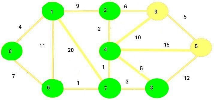
Let's say the vertex 0 is our starting point. We are going to set the initial costs of vertices in this graph like this:

We pick the vertex with a minimum cost - that vertex is 0. We will mark it as visited and add it to our set of visited vertices. The visited nodes will be marked with green color in the images:

Then, we will update the cost of adjacent vertices (1 and 6).

Since 0 + 4 < infinity and 0 + 7 < infinity, the new costs will be the following (the numbers in bold will be visited vertices):

Now we visit the next smallest cost node, which is 1.

We mark it as visited, and then update the adjacent vertices: 2, 6, and 7:

Since 4 + 9 < infinity, new cost of vertex 2 will be 13
Since 4 + 11 > 7, the cost of vertex 6 will remain 7
Since 4 + 20 < infinity

These are our new costs:

The next vertex we're going to visit is vertex 6. We mark it as visited and update its adjacent vertices' costs:

Since 7 + 1 < 24, the new cost for vertex 7 will be 8.

These are our new costs:

The next vertex we are going to visit is vertex 7:

Now we're going to update the adjacent vertices: vertices 4 and 8.

Since 8 + 1 < infinity, the new cost of vertex 4 is 9
Since 8 + 3 < infinity, the new cost of vertex 8 is 11

These are the new costs:

The next vertex we'll visit is vertex 4:

We will now update the adjacent vertices: 2, 3, 5, and 8.

Free eBook: Git Essentials

Check out our hands-on, practical guide to learning Git, with best-practices, industry-accepted standards, and included cheat sheet. Stop Googling Git commands and actually learn it!Download the eBook

Since 9 + 2 < 13, the new cost of vertex 2 is 11
Since 9 + 10 < infinity, the new cost of vertex 3 is 19
Since 9 + 15 < infinity

The new costs are:

The next vertex we are going to visit is vertex 2:

The only vertex we're going to update is vertex 3:

Since 11 + 6 > 19, the cost of vertex 3 stays the same

Therefore, the current costs for all nodes will stay the same as before.

The next vertex we are going to visit is vertex 8:

We are updating the vertex 5:

Since 11 + 12 < 24, the new cost of vertex 5 is going to be 23

The costs of vertices right now are:

The next vertex we are going to visit is vertex 3.

We are updating the remaining adjacent vertex - vertex 5.

Since 19 + 5 > 23, the cost of vertex 5 remains the same

The final vertex we are going to visit is vertex 5:

There are no more unvisited vertices that may need an update.

Our final costs represents the shortest paths from node 0 to every other node in the graph:

Implementation

Now that we've gone over an example, let's see how we can implement Dijkstra's algorithm in Python!

Before we start, we are first going to have to import a priority queue:

We will use a priority queue to easily sort the vertices we haven't visited yet, which will more easily allow us to choose the one of shortest current cost.

Now, we'll implement a constructor for a class called Graph:

In this simple parametrized constructor, we provided the number of vertices in the graph as an argument, and we initialized three fields:

v: Represents the number of vertices in the graph
edges: Represents the list of edges in the form of a matrix. For nodes u and v, self.edges[u][v] = weight of the edge

Now, let's define a function which is going to add an edge to a graph:

Now, let's write the function for Dijkstra's algorithm:

In this code, we first created a list D of the size v. The entire list is initialized to infinity. This is going to be a list where we keep the shortest paths from start_vertex to all of the other nodes.

We set the value of the start vertex to 0, since that is its distance from itself.

Then, we initialize a priority queue, which we will use to quickly sort the vertices from the least to most distant. We put the start vertex in the priority queue.

Now, for each vertex in the priority queue, we will first mark them as visited, and then we will iterate through their neighbors.

If the neighbor is not visited, we will compare its old cost and its new cost.

The old cost is the current value of the shortest path from the start vertex to the neighbor, while the new cost is the value of the sum of the shortest path from the start vertex to the current vertex and the distance between the current vertex and the neighbor.

If the new cost is lower than the old cost, we put the neighbor and its cost to the priority queue, and update the list where we keep the shortest paths accordingly.

Finally, after all of the vertices are visited and the priority queue is empty, we return the list D. Our function is done!

Let's put the graph we used in the example above as the input of our implemented algorithm:

BFS

from .count_islands import *
from .maze_search import

BFS Examples

Dijkstra's algorithm

Introduction

In computer science (as well as in our everyday life), there are a lot of problems that require finding the shortest path between two points. We encounter problems such as:

Finding the shortest path from our house to our school or workplace
Finding the quickest way to get to a gas station while traveling
Finding a list of friends that a particular user on social network may know

These are just a few of the many "shortest path problems" we see daily. Dijkstra's algorithm is one of the most well known shortest path algorithms because of it's efficiency and simplicity.

Graphs and Types of Graphs

Dijkstra's algorithm works on undirected, connected, weighted graphs. Before we get into it, let's explain what an undirected, connected, and weighed graph actually is.

A graph is a data structure represented by two things:

Vertices: Groups of certain objects or data (also known as a "node")
Edges: Links that connect those groups of objects or data

One more example of a graph can be a circle route of a train: the train stations are represented by vertices, and the rails between them are represented by the edges of a graph.

Graphs can be divided based on the types of their edges or based on the number of components that represent them.

When it comes to their edges, graphs can be:

Directed
Undirected

Another division by the edges in a graph can be:

Weighted
Unweighted

An unweighted graph is a graph whose edges don't have weights, like the forementioned graph of relationships between people - we can't assign a numerical value to "knowing a person"!

Based on the number of components that represent them, graphs can be:

Connected
Disconnected

Dijkstra's Algorithm

We will now go over this algorithm step by step:

First, we will create a set of visited vertices, to keep track of all of the vertices that have been assigned their correct shortest path.
We will also need to set "costs" of all vertices in the graph (lengths of the current shortest path that leads to it). All of the costs will be set to 'infinity' at the begining, to make sure that every other cost we may compare it to would be smaller than the starting one. The only exception is the cost of the first, starting vertex - this vertex will have a cost of 0, because it has no path to itself.
As long as there are vertices without the shortest path assigned to them, we do the following:

Let's explain this a bit better using an example:

Let's say the vertex 0 is our starting point. We are going to set the initial costs of vertices in this graph like this:

We pick the vertex with a minimum cost - that vertex is 0. We will mark it as visited and add it to our set of visited vertices. The visited nodes will be marked with green color in the images:

Then, we will update the cost of adjacent vertices (1 and 6).

Since 0 + 4 < infinity and 0 + 7 < infinity, the new costs will be the following (the numbers in bold will be visited vertices):

Now we visit the next smallest cost node, which is 1.

We mark it as visited, and then update the adjacent vertices: 2, 6, and 7:

Since 4 + 9 < infinity, new cost of vertex 2 will be 13
Since 4 + 11 > 7, the cost of vertex 6 will remain 7
Since 4 + 20 < infinity

These are our new costs:

The next vertex we're going to visit is vertex 6. We mark it as visited and update its adjacent vertices' costs:

Since 7 + 1 < 24, the new cost for vertex 7 will be 8.

These are our new costs:

The next vertex we are going to visit is vertex 7:

Now we're going to update the adjacent vertices: vertices 4 and 8.

Since 8 + 1 < infinity, the new cost of vertex 4 is 9
Since 8 + 3 < infinity, the new cost of vertex 8 is 11

These are the new costs:

The next vertex we'll visit is vertex 4:

We will now update the adjacent vertices: 2, 3, 5, and 8.

Free eBook: Git Essentials

Since 9 + 2 < 13, the new cost of vertex 2 is 11
Since 9 + 10 < infinity, the new cost of vertex 3 is 19
Since 9 + 15 < infinity

The new costs are:

The next vertex we are going to visit is vertex 2:

The only vertex we're going to update is vertex 3:

Since 11 + 6 > 19, the cost of vertex 3 stays the same

Therefore, the current costs for all nodes will stay the same as before.

The next vertex we are going to visit is vertex 8:

We are updating the vertex 5:

Since 11 + 12 < 24, the new cost of vertex 5 is going to be 23

The costs of vertices right now are:

The next vertex we are going to visit is vertex 3.

We are updating the remaining adjacent vertex - vertex 5.

Since 19 + 5 > 23, the cost of vertex 5 remains the same

The final vertex we are going to visit is vertex 5:

There are no more unvisited vertices that may need an update.

Our final costs represents the shortest paths from node 0 to every other node in the graph:

Implementation

Now that we've gone over an example, let's see how we can implement Dijkstra's algorithm in Python!

Before we start, we are first going to have to import a priority queue:

We will use a priority queue to easily sort the vertices we haven't visited yet, which will more easily allow us to choose the one of shortest current cost.

Now, we'll implement a constructor for a class called Graph:

In this simple parametrized constructor, we provided the number of vertices in the graph as an argument, and we initialized three fields:

v: Represents the number of vertices in the graph
edges: Represents the list of edges in the form of a matrix. For nodes u and v, self.edges[u][v] = weight of the edge

Now, let's define a function which is going to add an edge to a graph:

Now, let's write the function for Dijkstra's algorithm:

We set the value of the start vertex to 0, since that is its distance from itself.

Then, we initialize a priority queue, which we will use to quickly sort the vertices from the least to most distant. We put the start vertex in the priority queue.

Now, for each vertex in the priority queue, we will first mark them as visited, and then we will iterate through their neighbors.

If the neighbor is not visited, we will compare its old cost and its new cost.

If the new cost is lower than the old cost, we put the neighbor and its cost to the priority queue, and update the list where we keep the shortest paths accordingly.

Finally, after all of the vertices are visited and the priority queue is empty, we return the list D. Our function is done!

Let's put the graph we used in the example above as the input of our implemented algorithm:

Calculate a Factorial With Python - Iterative and Recursive

Introduction

By definition, a factorial is the product of a positive integer and all the positive integers that are less than or equal to the given number. In other words, getting a factorial of a number means to multiply all whole numbers from that number, down to 1.

0! equals 1 as well, by convention.

A factorial is denoted by the integer and followed by an exclamation mark.

5! denotes a factorial of five.

And to calculate that factorial, we multiply the number with every whole number smaller than it, until we reach 1:

Keeping these rules in mind, in this tutorial, we will learn how to calculate the factorial of an integer with Python, using loops and recursion. Let's start with calculating the factorial using loops.

Calculating Factorial Using Loops

We can calculate factorials using both the while loop and the for loop. The general process is pretty similar for both. All we need is a parameter as input and a counter.

Let's start with the for loop:

You may have noticed that we are counting starting from 1 to the n, whilst the definition of factorial was from the given number down to 1. But mathematically:

1∗2∗3∗4...∗n=n∗(n−1)∗(n−2)∗(n−3)∗(n−4)...∗(n−(n−1))1∗2∗3∗4...∗n=n∗(n−1)∗(n−2)∗(n−3)∗(n−4)...∗(n−(n−1))

To simplify, (n - (n-1)) will always be equal to 1.

That means that it doesn't matter in which direction we're counting. It can start from 1 and increase towards the n, or it can start from n and decrease towards 1. Now that's clarified, let's start breaking down the function we've just wrote.

Our function takes in a parameter n which denotes the number we're calculating a factorial for. First, we define a variable named result and assign 1 as a value to it.

Why assign 1 and not 0 you ask?

Because if we were to assign 0 to it then all the following multiplications with 0, naturally would result in a huge 0.

Then we start our for loop in the range from 1 to n+1. Remember, the Python range will stop before the second argument. To include the last number as well, we simply add an additional 1.

Inside the for loop, we multiply the current value of result with the current value of our index i.

Finally, we return the final value of the result. Let's test our function print out the result:

If you'd like to read more about how to get user input, read our .

It will prompt the user to give input. We'll try it with 4:

You can use a calculator to verify the result:

4! is 4 * 3 * 2 * 1, which results 24.

Now let's see how we can calculate factorial using the while loop. Here's our modified function:

This is pretty similar to the for loop. Except for this time we're moving from n towards the 1, closer to the mathematical definition. Let's test our function:

We'll enter 4 as an input once more:

Although the calculation was 4 * 3 * 2 * 1 the final result is the same as before.

Calculating factorials using loops was easy. Now let's take a look at how to calculate the factorial using a recursive function.

Calculating Factorial Using Recursion

A recursive function is a function that calls itself. It may sound a bit intimidating at first but bear with us and you'll see that recursive functions are easy to understand.

In general, every recursive function has two main components: a base case and a recursive step.

Base cases are the smallest instances of the problem. Also a break, a case that will return a value and will get out of the recursion. In terms of factorial functions, the base case is when we return the final element of the factorial, which is 1.

Without a base case or with an incorrect base case, your recursive function can run infinitely, causing an overflow.

Recursive steps - as the name implies- are the recursive part of the function, where the whole problem is transformed into something smaller. If the recursive step fails to shrink the problem, then again recursion can run infinitely.

Consider the recurring part of the factorials:

5! is 5 * 4 * 3 * 2 * 1.

But we also know that:

4 * 3 * 2 * 1 is 4!.

In other words 5! is 5 * 4!, and 4! is 4 * 3! and so on.

So we can say that n! = n * (n-1)!. This will be the recursive step of our factorial!

A factorial recursion ends when it hits 1. This will be our base case. We will return 1 if n is 1 or less, covering the zero input.

Let's take a look at our recursive factorial function:

As you see the if block embodies our base case, while the else block covers the recursive step.

Let's test our function:

We will enter 3 as input this time:

We get the same result. But this time, what goes under the hood is rather interesting:

You see, when we enter the input, the function will check with the if block, and since 3 is greater than 1, it will skip to the else block. In this block, we see the line return n * get_factorial_recursively(n-1).

We know the current value of n for the moment, it's 3, but get_factorial_recursively(n-1) is still to be calculated.

Then the program calls the same function once more, but this time our function takes 2 as the parameter. It checks the if block and skips to the else block and again encounters with the last line. Now, the current value of the n is 2 but the program still must calculate the get_factorial_recursively(n-1).

So it calls the function once again, but this time the if block, or rather, the base class succeeds to return 1 and breaks out from the recursion.

Following the same pattern to upwards, it returns each function result, multiplying the current result with the previous n and returning it for the previous function call. In other words, our program first gets to the bottom of the factorial (which is 1), then builds its way up, while multiplying on each step.

Also removing the function from the call stack one by one, up until the final result of the n * (n-1) is returned.

This is generally how recursive functions work. Some more complicated problems may require deeper recursions with more than one base case or more than one recursive step. But for now, this simple recursion is good enough to solve our factorial problem!


"""
Climbing Staircase

There exists a staircase with N steps, and you can climb up either X different steps at a time.
Given N, write a function that returns the number of unique ways you can climb the staircase.
The order of the steps matters.

Input: steps = [1, 2], height = 4
Output: 5
Output explanation:
1, 1, 1, 1
2, 1, 1
1, 2, 1
1, 1, 2
2, 2

=========================================
Dynamic Programing solution.
    Time Complexity:    O(N*S)
    Space Complexity:   O(N)
"""


############
# Solution #
############


def climbing_staircase(steps, height):
    dp = [0 for i in range(height)]

    # add all steps into dp
    for s in steps:
        if s <= height:
            dp[s - 1] = 1

    # for each position look how you can arrive there
    for i in range(height):
        for s in steps:
            if i - s >= 0:
                dp[i] += dp[i - s]

    return dp[height - 1]


###########
# Testing #
###########

# Test 1
# Correct result => 5
print(climbing_staircase([1, 2], 4))

# Test 2
# Correct result => 3
print(climbing_staircase([1, 3, 5], 4))

"""
Coin Change

You are given coins of different denominations and a total amount of money amount.
Write a function to compute the fewest number of coins that you need to make up that amount.
If that amount of money cannot be made up by any combination of the coins, return -1.

Input: coins = [1, 2, 5], amount = 11
Output: 3

Input: coins = [2], amount = 3
Output: -1

=========================================
Dynamic programming solution 1
    Time Complexity:    O(A*C)  , A = amount, C = coins
    Space Complexity:   O(A)
Dynamic programming solution 2 (don't need the whole array, just use modulo to iterate through the partial array)
    Time Complexity:    O(A*C)  , A = amount, C = coins
    Space Complexity:   O(maxCoin)
"""


##############
# Solution 1 #
##############


def coin_change_1(coins, amount):
    if amount == 0:
        return 0
    if len(coins) == 0:
        return -1

    max_value = amount + 1  # use this instead of math.inf
    dp = [max_value for i in range(max_value)]
    dp[0] = 0

    for i in range(1, max_value):
        for c in coins:
            if c <= i:
                # search on previous positions for min coins needed
                dp[i] = min(dp[i], dp[i - c] + 1)

    if dp[amount] == max_value:
        return -1
    return dp[amount]


##############
# Solution 2 #
##############


def coin_change_2(coins, amount):
    if amount == 0:
        return 0
    if len(coins) == 0:
        return -1

    max_value = amount + 1
    max_coin = min(max_value, max(coins) + 1)
    dp = [max_value for i in range(max_coin)]
    dp[0] = 0

    for i in range(1, max_value):
        i_mod = i % max_coin
        dp[i_mod] = max_value  # reset current position

        for c in coins:
            if c <= i:
                # search on previous positions for min coins needed
                dp[i_mod] = min(dp[i_mod], dp[(i - c) % max_coin] + 1)

    if dp[amount % max_coin] == max_value:
        return -1
    return dp[amount % max_coin]


###########
# Testing #
###########

# Test 1
# Correct result => 3
coins = [1, 2, 5]
amount = 11
print(coin_change_1(coins, amount))
print(coin_change_2(coins, amount))

# Test 2
# Correct result => -1
coins = [2]
amount = 3
print(coin_change_1(coins, amount))
print(coin_change_2(coins, amount))

"""
Count IP Addresses

An IP Address (IPv4) consists of 4 numbers which are all between 0 and 255.
In this problem however, we are dealing with 'Extended IP Addresses' which consist of K such numbers.
Given a string S containing only digits and a number K,
your task is to count how many valid 'Extended IP Addresses' can be formed.
An Extended IP Address is valid if:
* it consists of exactly K numbers
* each numbers is between 0 and 255, inclusive
* a number cannot have leading zeroes

Input: '1234567', 3
Output: 1
Output explanation: Valid IP addresses: '123.45.67'.

Input: '100111', 3
Output: 1
Output explanation: Valid IP addresses: '100.1.11', '100.11.1', '10.0.111'.

Input: '345678', 2
Output: 0
Output explanation: It is not possible to form a valid IP Address with two numbers.

=========================================
1D Dynamic programming solution.
    Time Complexity:    O(N*K)
    Space Complexity:   O(N)
"""


############
# Solution #
############


def count_ip_addresses(S, K):
    n = len(S)
    if n == 0:
        return 0
    if n < K:
        return 0

    dp = [0] * (n + 1)
    dp[0] = 1

    for i in range(K):
        # if you want to save just little calculations you can use min(3*(i+1), n) instead of n
        for j in range(n, i, -1):
            # reset the value
            dp[j] = 0

            # use iteration to check all 3 possible numbers (x, xx, xxx), instead of writing 3 IFs
            for e in range(max(i, j - 3), j):
                if is_valid(S[e:j]):
                    dp[j] += dp[e]

    return dp[n]


def is_valid(S):
    if (len(S) > 1) and (S[0] == "0"):
        return False
    return int(S) <= 255


###########
# Testing #
###########

# Test 1
# Correct result => 1
print(count_ip_addresses("1234567", 3))

# Test 2
# Correct result => 3
print(count_ip_addresses("100111", 3))

# Test 3
# Correct result => 0
print(count_ip_addresses("345678", 2))

"""
Create Palindrome (Minimum Insertions to Form a Palindrome)

Given a string, find the palindrome that can be made by inserting the fewest number of characters as possible anywhere in the word.
If there is more than one palindrome of minimum length that can be made, return the lexicographically earliest one (the first one alphabetically).

Input: 'race'
Output: 'ecarace'
Output explanation: Since we can add three letters to it (which is the smallest amount to make a palindrome).
                    There are seven other palindromes that can be made from "race" by adding three letters, but "ecarace" comes first alphabetically.

Input: 'google'
Output: 'elgoogle'

Input: 'abcda'
Output: 'adcbcda'
Output explanation: Number of insertions required is 2 - aDCbcda (between the first and second character).

Input: 'adefgfdcba'
Output: 'abcdefgfedcba'
Output explanation: Number of insertions required is 3 i.e. aBCdefgfEdcba.

=========================================
Recursive count how many insertions are needed, very slow and inefficient.
    Time Complexity:    O(2^N)
    Space Complexity:   O(N^2)  , for each function call a new string is created (and the recursion can have depth of max N calls)
Dynamic programming. Count intersections looking in 3 direction in the dp table (diagonally left-up or min(left, up)).
    Time Complexity:    O(N^2)
    Space Complexity:   O(N^2)
"""


##############
# Solution 1 #
##############


def create_palindrome_1(word):
    n = len(word)

    # base cases
    if n == 1:
        return word
    if n == 2:
        if word[0] != word[1]:
            word += word[0]  # make a palindrom
        return word

    # check if the first and last chars are same
    if word[0] == word[-1]:
        # add first and last chars
        return word[0] + create_palindrome_1(word[1:-1]) + word[-1]

    # if not remove the first and after that the last char
    # and find which result has less chars
    first = create_palindrome_1(word[1:])
    first = word[0] + first + word[0]  # add first char twice

    last = create_palindrome_1(word[:-1])
    last = word[-1] + last + word[-1]  # add last char twice

    if len(first) < len(last):
        return first
    return last


##############
# Solution 2 #
##############

import math


def create_palindrome_2(word):
    n = len(word)
    dp = [[0 for j in range(n)] for i in range(n)]

    # run dp
    for gap in range(1, n):
        left = 0
        for right in range(gap, n):
            if word[left] == word[right]:
                dp[left][right] = dp[left + 1][right - 1]
            else:
                dp[left][right] = min(dp[left][right - 1], dp[left + 1][right]) + 1
            left += 1

    # build the palindrome using the dp table
    return build_palindrome(word, dp, 0, n - 1)


def build_palindrome(word, dp, left, right):
    # similar like the first solution, but without exponentialy branching
    # this is linear time, we already know the inserting values
    if left > right:
        return ""
    if left == right:
        return word[left]

    if word[left] == word[right]:
        return word[left] + build_palindrome(word, dp, left + 1, right - 1) + word[left]

    if dp[left + 1][right] < dp[left][right - 1]:
        return word[left] + build_palindrome(word, dp, left + 1, right) + word[left]

    return word[right] + build_palindrome(word, dp, left, right - 1) + word[right]


###########
# Testing #
###########

# Test 1
# Correct result => 'ecarace'
word = "race"
print(create_palindrome_1(word))
print(create_palindrome_2(word))

# Test 2
# Correct result => 'elgoogle'
word = "google"
print(create_palindrome_1(word))
print(create_palindrome_2(word))

# Test 3
# Correct result => 'adcbcda'
word = "abcda"
print(create_palindrome_1(word))
print(create_palindrome_2(word))

# Test 4
# Correct result => 'abcdefgfedcba'
word = "adefgfdcba"
print(create_palindrome_1(word))
print(create_palindrome_2(word))

"""
Interleaving Strings

Given are three strings A, B and C.
C is said to be interleaving of A and B, if:
- it contains all characters of A and B, and
- order of all characters from A and B is preserved in C
Your task is to count in how many ways C can be formed by interleaving of A and B.

Input: A='xy', B= 'xz', C: 'xxyz'
Output: 2
Output explanation: 
    1) Take 'x' from A, then 'x' from B, then 'y' from A and at the end 'z' from B.
    2) Take 'x' from B, then 'x' from A, then 'y' from A and at the end 'z' from B.

=========================================
2D Dynamic programming solution.
    Time Complexity:    O(N*M)
    Space Complexity:   O(N*M)
1D Dynamic programming solution. Only the last two rows from the whole matrix are used, but that could be represented using only 1 row.
    Time Complexity:    O(N*M)
    Space Complexity:   O(M)
"""

##############
# Solution 1 #
##############


def interleaving_strings_1(A, B, C):
    nA, nB, nC = len(A), len(B), len(C)
    if nA + nB != nC:
        return 0

    dp = [[0 for j in range(nB + 1)] for i in range(nA + 1)]

    # starting values
    dp[0][0] = 1

    for i in range(1, nA + 1):
        if A[i - 1] == C[i - 1]:
            # short form of if A[i - 1] == C[i - 1] and dp[i - 1][0] == 1
            # dp[i][0] and dp[0][1] can be only 0 or 1
            dp[i][0] = dp[i - 1][0]

    for i in range(1, nB + 1):
        if B[i - 1] == C[i - 1]:
            dp[0][i] = dp[0][i - 1]

    # run dp
    for i in range(1, nA + 1):
        for j in range(1, nB + 1):
            if A[i - 1] == C[i + j - 1]:
                # look for the dp value from the previous position
                dp[i][j] += dp[i - 1][j]
            if B[j - 1] == C[i + j - 1]:
                # look for the dp value from the previous position
                dp[i][j] += dp[i][j - 1]

    return dp[nA][nB]


##############
# Solution 2 #
##############


def interleaving_strings_2(A, B, C):
    nA, nB, nC = len(A), len(B), len(C)
    if nA + nB != nC:
        return 0

    dp = [0 for j in range(nB + 1)]

    # starting values
    dp[0] = 1

    for i in range(1, nB + 1):
        if B[i - 1] == C[i - 1]:
            dp[i] = dp[i - 1]

    # run dp
    for i in range(1, nA + 1):
        if A[i - 1] != C[i - 1]:
            # reset the value
            dp[0] = 0

        for j in range(1, nB + 1):
            if A[i - 1] != C[i + j - 1]:
                # reset the value
                dp[j] = 0
            if B[j - 1] == C[i + j - 1]:
                dp[j] += dp[j - 1]

    return dp[nB]


###########
# Testing #
###########

# Test 1
# Correct result => 2
a, b, c = "xy", "xz", "xxyz"
print(interleaving_strings_1(a, b, c))
print(interleaving_strings_2(a, b, c))

"""
Jump Game 2

Given an array of non-negative integers, you are initially positioned at the first index of the array.
Each element in the array represents your maximum jump length at that position.
Your goal is to reach the last index in the minimum number of jumps.

Input: XXX
Output: XXX
Output explanation: XXX

=========================================
Classical 1D Dynamic Programming solution.
    Time Complexity:    O(N)    , maybe looks like O(N^2) but that's not possible
    Space Complexity:   O(N)
If you analyze the previous solution, you'll see that you don't need the whole DP array.
    Time Complexity:    O(N)
    Space Complexity:   O(1)
"""


##############
# Solution 1 #
##############


def min_jumps_1(nums):
    n = len(nums)
    if n <= 1:
        return 0

    dp = [-1] * n
    dp[0] = 0

    for i in range(n):
        this_jump = i + nums[i]
        jumps = dp[i] + 1

        if this_jump >= n - 1:
            return jumps

        # starging from back, go reverse and
        # change all -1 values and break when first positive is found
        for j in range(this_jump, i, -1):
            if dp[j] != -1:
                break
            dp[j] = jumps


##############
# Solution 2 #
##############


def min_jumps_2(nums):
    n = len(nums)
    if n <= 1:
        return 0

    jumps = 0
    max_jump = 0
    new_max_jump = 0

    for i in range(n):
        if max_jump < i:
            max_jump = new_max_jump
            jumps += 1

        this_jump = i + nums[i]
        if this_jump >= n - 1:
            return jumps + 1

        new_max_jump = max(new_max_jump, this_jump)


###########
# Testing #
###########

# Test 1
# Correct result => 2
nums = [2, 3, 1, 1, 4]
print(min_jumps_1(nums))
print(min_jumps_2(nums))

"""
Longest Common Subsequence

Given 2 strings, find the longest common subseqence - https://en.wikipedia.org/wiki/Longest_common_subsequence_problem
NOT Longest Common Substring, this is a different problem.
Substring is a string composed ONLY of neighboring chars, subsequence could contain non-neighboring chars.

Input: 'ABAZDC', 'BACBAD'
Output: 'ABAD'

Input: 'I'm meto', 'I am Meto'
Output: 'Im eto'

=========================================
Dynamic programming solution.
Find more details here: https://www.geeksforgeeks.org/printing-longest-common-subsequence/
    Time Complexity:    O(N * M)
    Space Complexity:   O(N * M)    , can be O(M) see longest_common_substring.py solution (but you'll need to save subsequences)
"""


############
# Solution #
############


def longest_common_subsequence(str1, str2):
    n, m = len(str1), len(str2)
    # create dp matrix
    dp = [[0 for j in range(m + 1)] for i in range(n + 1)]

    # run dp
    for i in range(1, n + 1):
        for j in range(1, m + 1):
            # checks only in 3 directions in the table
            # in short: to the current position dp could come from those 3 previous positions
            #   ^  ^
            #    \ |
            #   <- O
            if str1[i - 1] == str2[j - 1]:
                # from this position dp could come only if there is a match in the previous chars
                dp[i][j] = dp[i - 1][j - 1] + 1
            else:
                # dp could come from these positions only if there is no much
                dp[i][j] = max(dp[i - 1][j], dp[i][j - 1])

    # find the subseqence/string
    letters = dp[n][m]
    # use an array for storing the chars because string manipulation operations are not time and space efficient
    result = ["" for i in range(letters)]
    i = n
    j = m

    while (i != 0) and (j != 0):
        # use the inverse logic from upper code (filling the dp table)
        if str1[i - 1] == str2[j - 1]:
            letters -= 1
            result[letters] = str1[i - 1]
            j -= 1
            i -= 1
        elif dp[i - 1][j] < dp[i][j - 1]:
            j -= 1
        else:
            i -= 1

    return "".join(result)


###########
# Testing #
###########

# Test 1
# Correct result => 'ABAD'
print(longest_common_subsequence("ABAZDC", "BACBAD"))

# Test 2
# Correct result => 'Im eto'
print(longest_common_subsequence("I'm meto", "I am Meto"))

"""
Longest Common Substring

Given two strings X and Y, find the of longest common substring.

Input: 'GeeksforGeeks', 'GeeksQuiz'
Output: 'Geeks'

=========================================
Dynamic Programming Solution.
    Time Complexity:    O(N * M)
    Space Complexity:   O(M)
* For this problem exists a faster solution, using Suffix tree, Time Complexity O(N + M).
"""


############
# Solution #
############


def longest_common_substring(str1, str2):
    n, m = len(str1), len(str2)
    # instead of creating a whole dp table, use only 2 rows (current and previous row)
    curr = [0 for j in range(m + 1)]
    prev = []
    max_length = 0
    max_idx = 0

    for i in range(1, n + 1):
        # save the previous row and create the current row
        prev = curr
        curr = [0 for j in range(m + 1)]

        for j in range(1, m + 1):
            if str1[i - 1] == str2[j - 1]:
                # search only for matching chars
                curr[j] = prev[j - 1] + 1

                if curr[j] > max_length:
                    # save the last matching index of the first string
                    max_length = curr[j]
                    max_idx = i

    return str1[max_idx - max_length : max_idx]


###########
# Testing #
###########

# Test 1
# Correct result => BABC
print(longest_common_substring("ABABC", "BABCA"))

# Test 2
# Correct result => Geeks
print(longest_common_substring("GeeksforGeeks", "GeeksQuiz"))

# Test 3
# Correct result => abcd
print(longest_common_substring("abcdxyz", "xyzabcd"))

# Test 4
# Correct result => abcdez
print(longest_common_substring("zxabcdezy", "yzabcdezx"))

"""
Longest Increasing Subsequence (LIS)

Find the longest increasing subsequence.
(subsequence doesn't mean that all elements need to be neighboring in the original array).

Sample input: [1, 4, 2, 0, 3, 1]
Sample output: [1, 2, 3]
or output the length
Sample output: 3

=========================================
Dynamic programming (classical) solution.
    Time Complexity:    O(N^2)
    Space Complexity:   O(N)
Dynamic programing in combination with binary search.
Explanation in details: https://www.geeksforgeeks.org/longest-monotonically-increasing-subsequence-size-n-log-n/
    Time Complexity:    O(N * logN)
    Space Complexity:   O(N^2)      , if you need only the length of the LIS, extra space complexity will be O(N)
"""


##############
# Solution 1 #
##############


def longest_increasing_subsequence_1(nums):
    n = len(nums)
    if n == 0:
        return 0
    dp = [1 for i in range(n)]
    max_val = 1

    # run dp
    for i in range(n):
        for j in range(i):
            if nums[j] < nums[i]:
                dp[i] = max(dp[i], dp[j] + 1)
                max_val = max(max_val, dp[i])

    # find the values (there could be more combinations/solutions)
    current_val = max_val
    result = [0 for i in range(current_val)]
    # start from the back and look for the biggest value in dp list
    for i in range(n - 1, -1, -1):
        if (dp[i] == current_val) and (
            (len(result) == current_val) or (result[current_val] > nums[i])
        ):
            current_val -= 1
            result[current_val] = nums[i]

    return result


##############
# Solution 2 #
##############


def longest_increasing_subsequence_2(nums):
    n = len(nums)
    if n == 0:
        return 0
    # the last dp array result in longest increasing subsequence
    dp = []

    for i in range(n):
        idx = binary_search(dp, nums[i])
        k = len(dp)

        if idx == k:
            # bigger element than the current wasn't found
            arr = []
            if k != 0:
                arr = [i for i in dp[-1]]  # make a copy
            arr.append(nums[i])

            dp.append(arr)
        elif dp[idx][-1] > nums[i]:
            # smaller element was found, replace it
            dp[idx][-1] = nums[i]

    return dp[-1]


def binary_search(dp, target):
    l = 0
    r = len(dp) - 1

    while l <= r:
        mid = l + (r - l) // 2
        if dp[mid][-1] == target:
            return mid
        elif dp[mid][-1] < target:
            l = mid + 1
        else:
            r = mid - 1

    return l


###########
# Testing #
###########

# Test 1
# Correct result => [2, 3, 7, 18] - one of the possible combinations
arr = [10, 9, 2, 5, 3, 7, 101, 18]
print(longest_increasing_subsequence_1(arr))
print(longest_increasing_subsequence_2(arr))

# Test 2
# Correct result => [1, 2, 3]
arr = [1, 2, 3]
print(longest_increasing_subsequence_1(arr))
print(longest_increasing_subsequence_2(arr))

# Test 3
# Correct result => [1, 2, 5, 7, 12] - one of the possible combinations
arr = [10, 1, 3, 8, 2, 0, 5, 7, 12, 3]
print(longest_increasing_subsequence_1(arr))
print(longest_increasing_subsequence_2(arr))

# Test 4
# Correct result => [1, 2, 3, 4, 5, 6]
arr = [12, 1, 11, 2, 10, 3, 9, 4, 8, 5, 7, 6]
print(longest_increasing_subsequence_1(arr))
print(longest_increasing_subsequence_2(arr))

# Test 5
# Correct result => [1, 2, 3]
arr = [1, 4, 2, 0, 3, 1]
print(longest_increasing_subsequence_1(arr))
print(longest_increasing_subsequence_2(arr))

# Test 6
# Correct result => [3] - one of the possible combinations
arr = [7, 5, 5, 5, 5, 5, 3]
print(longest_increasing_subsequence_1(arr))
print(longest_increasing_subsequence_2(arr))

"""
Max Profit With K Transactions

You are given an array of integers representing the prices of a single stock on various days
(each index in the array represents a different day).
You are also given an integer k, which represents the number of transactions you are allowed to make.
One transaction consists of buying the stock on a given day and selling it on another, later day.
Write a function that returns the maximum profit that you can make buying and selling the stock,
given k transactions. Note that you can only hold 1 share of the stock at a time; in other words,
you cannot buy more than 1 share of the stock on any given day, and you cannot buy a share of the
stock if you are still holding another share.
In a day, you can first sell a share and buy another after that.

Input: [5, 11, 3, 50, 60, 90], 2
Output: 93
Output explanation: Buy 5, Sell 11; Buy 3, Sell 90

=========================================
Optimized dynamic programming solution.
For this solution you'll need only the current and previous rows.
The original (not optimized) DP formula is: MAX(dp[t][d-1], price[d] + MAX(dp[t-1][x] - price[x])),
but this is O(K * N^2) Time Complexity, and O(N * K) space complexity.
    Time Complexity:    O(N * К)
    Space Complexity:   O(N)
"""


############
# Solution #
############

import math


def max_profit_with_k_transactions(prices, k):
    days = len(prices)
    if days < 2:
        # not enough days for a transaction
        return 0

    # transaction = buy + sell (2 separate days)
    # in a day you can sell and after that buy a share
    # (according to this, can't exists more transactions than the number of the prices/days)
    k = min(k, days)
    # create space optimized dp matrix
    dp = [[0 for j in range(days)] for i in range(2)]

    for t in range(k):
        max_prev = -math.inf

        # compute which row is previous and which is the current one
        prev_idx = (t - 1) % 2
        curr_idx = t % 2

        # the values in dp table for these days will be same
        # just ignore them, don't update them (because those combinations were tried)
        past_days = t
        # only save the last one
        dp[curr_idx][past_days] = dp[prev_idx][past_days]

        for d in range(past_days + 1, days):
            # first try to buy with the current price
            max_prev = max(max_prev, dp[prev_idx][d - 1] - prices[d - 1])
            # after that try to sell with the current price
            dp[curr_idx][d] = max(dp[curr_idx][d - 1], max_prev + prices[d])

    # return the last value from the last transaction
    return dp[(k - 1) % 2][-1]


###########
# Testing #
###########

# Test 1
# Correct result => 9
print(max_profit_with_k_transactions([1, 2, 3, 4, 5, 6, 7, 8, 9, 10], 10))

# Test 2
# Correct result => 93
print(max_profit_with_k_transactions([5, 11, 3, 50, 60, 90], 2))

"""
Maximum subarray sum

The subarray must be contiguous.

Sample input: [-2, -3, 4, -1, -2, 1, 5, -3]
Sample output: 7
Output explanation: [4, -1, -2, 1, 5]

=========================================
Need only one iteration, in each step add the current element to the current sum.
When the sum is less than 0, reset the sum to 0 and continue with adding. (we care only about non-negative sums)
After each addition, check if the current sum is greater than the max sum. (Called Kadane's algorithm)
    Time Complexity:    O(N)
    Space Complexity:   O(1)
"""


############
# Solution #
############


def max_subarray_sum(a):
    curr_sum = 0
    max_sum = 0

    for val in a:
        # extend the current sum with the curren value;
        # reset it to 0 if it is smaller than 0, we care only about non-negative sums
        curr_sum = max(0, curr_sum + val)

        # check if this is the max sum
        max_sum = max(max_sum, curr_sum)

    return max_sum


###########
# Testing #
###########

# Test 1
# Correct result => 7
print(max_subarray_sum([-2, -3, 4, -1, -2, 1, 5, -3]))

# Test 2
# Correct result => 5
print(max_subarray_sum([1, -2, 2, -2, 3, -2, 4, -5]))

# Test 3
# Correct result => 7
print(max_subarray_sum([-2, -5, 6, -2, -3, 1, 5, -6]))

# Test 4
# Correct result => 0
print(max_subarray_sum([-6, -1]))

"""
Min Cost Coloring

A builder is looking to build a row of N houses that can be of K different colors.
He has a goal of minimizing cost while ensuring that no two neighboring houses are of the same color.
Given an N by K matrix where the nth row and kth column represents the cost to build the
nth house with kth color, return the minimum cost which achieves this goal.

=========================================
Dynamic programming, for each house search for the cheapest combination of the previous houses.
But don't search the whole array with combinations (colors), save only the smallest 2
(in this case we're sure that the previous house doesn't have the same color).
    Time Complexity:    O(N * K)
    Space Complexity:   O(1)
"""

############
# Solution #
############

import math


def min_cost_coloring(dp):
    # no need from a new dp matrix, you can use the input matrix
    n = len(dp)
    if n == 0:
        return 0
    m = len(dp[0])
    if m < 2:
        return -1

    # save only the smallest 2 costs instead of searching the whole previous array
    prev_min = [(0, -1), (0, -1)]

    for i in range(n):
        curr_min = [(math.inf, -1), (math.inf, -1)]

        for j in range(m):
            # find result with different color
            if j != prev_min[0][1]:
                dp[i][j] += prev_min[0][0]
            else:
                dp[i][j] += prev_min[1][0]

            # save the current result if smaller than the current 2
            if curr_min[0][0] > dp[i][j]:
                curr_min[1] = curr_min[0]
                curr_min[0] = (dp[i][j], j)
            elif curr_min[1][0] > dp[i][j]:
                curr_min[1] = (dp[i][j], j)

        prev_min = curr_min

    # return the min cost of the last house
    return min(dp[n - 1])


###########
# Testing #
###########

# Test 1
# Correct result => 5
print(
    min_cost_coloring(
        [[1, 2, 3, 4, 5], [5, 4, 3, 2, 1], [3, 2, 1, 4, 5], [3, 2, 1, 4, 3]]
    )
)

# Test 2
# Correct result => 6
print(
    min_cost_coloring(
        [[1, 2, 3, 4, 5], [1, 2, 3, 4, 5], [1, 2, 3, 4, 5], [1, 2, 3, 4, 5]]
    )
)

"""
Number of Decodings

Given the mapping a=1, b=2, ... , z=26, and an encoded message, count the number of ways it can be decoded.
For example, the message "111" would give 3, since it could be decoded as "aaa", "ka" and "ak".
All of the messages are decodable!

=========================================
The easiest solution is Brute-Force (building a tree and making all combinations),
and in the worst case there will be Fibbionaci(N) combinations, so the worst Time Complexity will be O(Fib(N))

Dynamic programming solution. Similar to number_of_smses.py.
    Time Complexity:    O(N)
    Space Complexity:   O(N)
"""


############
# Solution #
############


def num_decodings(code):
    n = len(code)
    dp = [0 for i in range(n)]

    if n == 0:
        return 0
    dp[0] = 1
    if n == 1:
        return dp[0]
    dp[1] = (code[1] != "0") + is_valid(code[0:2])

    for i in range(2, n):
        if code[i] != "0":
            # looking for how many combinations are there till now if this is a single digit
            dp[i] += dp[i - 1]
        if is_valid(code[i - 1 : i + 1]):
            # looking for how many combinations are there till now if this is a number of 2 digits
            dp[i] += dp[i - 2]

    return dp[n - 1]


def is_valid(code):
    k = int(code)
    return (k < 27) and (k > 9)


###########
# Testing #
###########

# Test 1
# Correct result => 5
print(num_decodings("12151"))

# Test 2
# Correct result => 5
print(num_decodings("1111"))

# Test 3
# Correct result => 3
print(num_decodings("111"))

# Test 4
# Correct result => 1
print(num_decodings("1010"))

# Test 5
# Correct result => 4
print(num_decodings("2626"))

# Test 6
# Correct result => 1
print(num_decodings("1"))

# Test 7
# Correct result => 2
print(num_decodings("11"))

# Test 8
# Correct result => 3
print(num_decodings("111"))

# Test 9
# Correct result => 5
print(num_decodings("1111"))

# Test 10
# Correct result => 8
print(num_decodings("11111"))

# Test 11
# Correct result => 13
print(num_decodings("111111"))

# Test 12
# Correct result => 21
print(num_decodings("1111111"))

# Test 13
# Correct result => 34
print(num_decodings("11111111"))

"""
Number of SMSes

Given the number sequence that is being typed in order to write and SMS message, return the count
of all the possible messages that can be constructed.

 1    2    3
     abc  def

 4    5    6
ghi  jkl  mno

 7    8    9
pqrs tuv wxyz

The blank space character is constructed with a '0'.

Input: '222'
Output: 4
Output explanation: '222' could mean: 'c', 'ab','ba' or 'aaa'. That makes 4 possible messages.

=========================================
Dynamic programming solution. Similar to number_of_decodings.py.
    Time Complexity:    O(N)
    Space Complexity:   O(N)
"""


############
# Solution #
############


def num_smses(sequence):
    n = len(sequence)
    dp = [0] * n

    # dp starting values, check all 4 possible starting combinations
    for i in range(min(4, n)):
        if is_valid(sequence[0 : i + 1]):
            dp[i] = 1

    # run dp
    for i in range(1, n):
        # check all 4 possible combinations (x, xx, xxx, xxxx)
        for j in range(min(4, i)):
            if is_valid(sequence[i - j : i + 1]):
                dp[i] += dp[i - j - 1]

    return dp[n - 1]


def is_valid(sequence):
    ch = sequence[0]

    for c in sequence:
        if c != ch:
            return False

    if sequence == "0":
        return True

    if ((ch >= "2" and ch <= "6") or ch == "8") and (len(sequence) < 4):
        return True

    if (ch == "7") or (ch == "9"):
        return True

    return False


###########
# Testing #
###########

# Test 1
# Correct result => 4
print(num_smses("222"))

# Test 2
# Correct result => 14
print(num_smses("2202222"))

# Test 3
# Correct result => 274
print(num_smses("2222222222"))

"""
Ordered Digits

We are given a number and we need to transform to a new number where all its digits are ordered in a non descending order.
We are allowed to increase or decrease a digit by 1, and each of those actions counts as one operation.
We are also allowed to over/underflow a number meaning from '9' we can change to '0' and also from '0' to '9', also costing only one operation.
One same digit can be changed multiple times.
Find the minimum number of operations we need to do do to create a new number with its ordered digits.

Input: 301
Output: 3
Output explanation: 301 -> 201 -> 101 -> 111, in this case 3 operations are required to get an ordered number.

Input: 901
Output: 1
Output explanation: 901 -> 001, in this case 1 operation is required to get an ordered number.

Input: 5982
Output: 4
Output explanation: 5982 -> 5981 -> 5980 -> 5989 -> 5999, in this case 4 operations are required to get an ordered number.

=========================================
Dynamic programming solution. For each position, calculate the cost of transformation to each possible digit (0-9).
And take the minimum value from the previous position (but smaller than the current digit).
    Time Complexity:    O(N)    , O(N*10) = O(N), N = number of digits
    Space Complexity:   O(N)    , same O(N*2) = O(N)
"""


############
# Solution #
############


def ordered_digits(number):
    n = len(number)
    dp = [[0 for j in range(10)] for i in range(2)]

    for i in range(n):
        min_prev = float("inf")
        for j in range(10):
            # find the min value from the previous digit and add it to the current value
            min_prev = min(min_prev, dp[(i - 1) % 2][j])
            # compute diff between the current digit and wanted digit
            diff = abs(j - int(number[i]))
            dp[i % 2][j] = min(diff, 10 - diff) + min_prev

    # min value from the last digit
    return min(dp[(n - 1) % 2])


###########
# Testing #
###########

# Test 1
# Correct result => 3
print(ordered_digits("301"))

# Test 2
# Correct result => 1
print(ordered_digits("901"))

# Test 3
# Correct result => 4
print(ordered_digits("5982"))

"""
Split Coins

You have a number of coins with various amounts.
You need to split the coins in two groups so that the difference between those groups in minimal.

Input: [1, 1, 1, 3, 5, 10, 18]
Output: 1
Output explanation: First group 1, 3, 5, 10 (or 1, 1, 3, 5, 10) and second group 1, 1, 18 (or 1, 18).

=========================================
Simple dynamic programming solution. Find the closest sum to the half of the sum of all coins.
    Time Complexity:    O(C*HS)     , C = number of coins, HS = half of the sum of all coins
    Space Complexity:   O(HS)
"""


############
# Solution #
############


def split_coins(coins):
    if len(coins) == 0:
        return -1

    full_sum = sum(coins)
    half_sum = full_sum // 2 + 1

    dp = [False] * half_sum
    dp[0] = True

    for c in coins:
        for i in range(half_sum - 1, -1, -1):
            if (i >= c) and dp[i - c]:
                # if you want to find coins, save the coin here dp[i] = c
                dp[i] = True

    for i in range(half_sum - 1, -1, -1):
        if dp[i]:
            # if you want to print coins, while i>0: print(dp[i]) i -= dp[i]
            return full_sum - 2 * i

    # not possible
    return -1


###########
# Testing #
###########

# Test 1
# Correct result => 1
print(split_coins([1, 1, 1, 3, 5, 10, 18]))

"""
Sum of non-adjacent numbers

Given a list of integers, write a function that returns the largest sum of non-adjacent numbers.
Numbers can be 0 or negative.

Input: [2, 4, 6, 2, 5]
Output: 13
Output explanation: We pick 2, 6, and 5.

Input: [5, 1, 1, 5]
Output: 10
Output explanation: We pick 5 and 5.

=========================================
Dynamic programming solution, but don't need the whole DP array, only the last 3 sums (DPs) are needed.
    Time Complexity:    O(N)
    Space Complexity:   O(1)
"""


############
# Solution #
############


def sum_non_adjacent(arr):
    n = len(arr)
    # from the dp matrix you only need the last 3 sums
    sums = [0, 0, 0]

    # TODO: refactor these if-elses, those are to skip using of DP matrix
    if n == 0:
        return 0

    # if negative or zero, the sum will be 0
    sums[0] = max(arr[0], 0)

    if n == 1:
        return sums[0]

    sums[1] = arr[1]
    # if the second number is negative or zero, then jump it
    if sums[1] <= 0:
        sums[1] = sums[0]

    if n == 2:
        return max(sums[0], sums[1])

    sums[2] = arr[2]
    # if the third number is negative or zero, then jump it
    if sums[2] <= 0:
        sums[2] = max(sums[0], sums[1])
    else:
        sums[2] += sums[0]

    # THE SOLUTION
    for i in range(3, n):
        temp = 0

        if arr[i] > 0:
            # take this number, because it's positive and the sum will be bigger
            temp = max(sums[0], sums[1]) + arr[i]
        else:
            # don't take this number, because the sum will be same or smaller
            temp = max(sums)

        # remove the first sum
        sums = sums[1:] + [temp]

    # return the max sum
    return max(sums)


###########
# Testing #
###########

# Test 1
# Correct result => 13
print(sum_non_adjacent([2, 4, 6, 2, 5]))

# Test 2
# Correct result => 15
print(sum_non_adjacent([2, 4, 2, 6, 2, -3, -2, 0, -3, 5]))

# Test 3
# Correct result => 10
print(sum_non_adjacent([5, 1, 1, 5]))

# Test 4
# Correct result => 10
print(sum_non_adjacent([5, 1, -1, 1, 5]))

"""
Transform Number Ascending Digits

Given a number and we need to transform to a new number where all its digits are ordered in a non descending order.
All digits can be increased, decreased, over/underflow are allowed.
Find the minimum number of operations we need to do to create a new number with its ordered digits.

Input: '5982'
Output: 4
Output explanation: 5999, 1 operation to transform 8 to 9, 3 operations to transform 2 to 9.

=========================================
Dynamic programming solution.
    Time Complexity:    O(N)    , O(N * 10 * 10) = O(100 N) = O(N)
    Space Complexity:   O(1)    , O(10 * 10) = O(100) = O(1)
"""


############
# Solution #
############


def operations(number):
    n = len(number)
    diff = lambda i, j: abs(j - int(number[i]))
    # compute diff between the current digit and wanted digit, and fill the dp
    prev_dp = [min(diff(0, i), 10 - diff(0, i)) for i in range(10)]

    # go through all digits and see all possible combinations using dynamic programming
    for i in range(1, n):
        curr_dp = [min(diff(i, j), 10 - diff(i, j)) for j in range(10)]
        for j in range(10):
            # find the min value for the previous digit and add it to the current value
            curr_dp[j] += min(prev_dp[0 : j + 1])
        prev_dp = curr_dp

    # min value from the last digit
    min_dist = min(prev_dp)

    return min_dist


###########
# Testing #
###########

# Test 1
# Correct result => 1
print(operations("901"))

# Test 2
# Correct result => 3
print(operations("301"))

# Test 3
# Correct result => 4
print(operations("5982"))

"""
Word Break (Find the original words)

Given a dictionary of words and a string made up of those words (no spaces), return the original sentence in a list.
If there is more than one possible reconstruction, return solution with less words.
If there is no possible reconstruction, then return null.

Input: sentence = 'thequickbrownfox', words = ['quick', 'brown', 'the', 'fox']
Output: ['the', 'quick', 'brown', 'fox']

Input: sentence = 'bedbathandbeyond', words = ['bed', 'bath', 'bedbath', 'and', 'beyond']
Output: ['bedbath', 'and', 'beyond'] (['bed', 'bath', 'and', 'beyond] has more words)

=========================================
Optimized dynamic programming solution (more simpler solutions can be found here https://www.geeksforgeeks.org/word-break-problem-dp-32/)
    Time Complexity:    O(N*M)  , N = number of chars in the sentence, M = max word length
    Space Complexity:   O(N+W)  , W = number of words
Bonus solution: Backtracking, iterate the sentence construct a substring and check if that substring exist in the set of words.
If the end is reached but the last word doesn't exist in the words, go back 1 word from the result (backtracking).
* But this solution doesn't give the result with the smallest number of words (gives the first found result)
    Time Complexity:    O(?)    , (worst case, about O(W! * N), for example sentence='aaaaaac', words=['a','aa','aaa','aaaa','aaaaa', 'aaaaaa'])
    Space Complexity:   O(W)
"""


############
# Solution #
############

import math


def word_break(sentence, words):
    n, w = len(sentence), len(words)
    if (n == 0) or (w == 0):
        return None

    dw = [-1 for i in range(n + 1)]
    dp = [math.inf for i in range(n + 1)]
    dp[0] = 0
    matched_indices = [0]

    dic = {}  # save all words in dictionary for faster searching
    max_word = 0  # length of the max word
    for i in range(w):
        dic[words[i]] = i
        max_word = max(max_word, len(words[i]))

    for i in range(1, n + 1):
        matched = False
        # start from the back of the matched_indices list (from the bigger numbers)
        for j in range(len(matched_indices) - 1, -1, -1):
            matched_index = matched_indices[j]
            # break this loop if the subsentence created with this matched index is bigger than the biggest word
            if matched_index < i - max_word:
                break

            subsentence = sentence[matched_index:i]
            # save this result if this subsentence exist in the words and number of words that forms sentence is smaller
            if (subsentence in dic) and (dp[matched_index] + 1 < dp[i]):
                dp[i] = dp[matched_index] + 1
                dw[i] = dic[subsentence]
                matched = True

        if matched:
            matched_indices.append(i)

    # the sentence can't be composed from the given words
    if dp[n] == math.inf:
        return None

    # find the words that compose this sentence
    result = ["" for i in range(dp[n])]
    i = n
    j = dp[n] - 1
    while i > 0:
        result[j] = words[dw[i]]
        i -= len(words[dw[i]])
        j -= 1

    return result


#########################
# Solution Backtracking #
#########################

from collections import deque


def word_break_backtracking(sentence, words):
    all_words = set()

    # create a set from all words
    for i in range(len(words)):
        all_words.add(words[i])

    n = len(sentence)
    i = 0
    subsentence = ""
    result = deque()

    # go letter by letter and save the new letter in subsentence
    while (i < n) or (len(subsentence) != 0):
        # if there are no left letters in the sentence, then this combination is not valid
        # remove the last word from the results and continue from that word
        if i == n:
            i -= len(subsentence)
            # if there are no words in the result, then this string is not composed only from the given words
            if len(result) == 0:
                return None
            subsentence = result[-1]
            result.pop()

        # add the new letter into subsentence and remove it from the sentence
        subsentence += sentence[i]
        i += 1

        # check if the new word exist in the set
        if subsentence in all_words:
            result.append(subsentence)
            subsentence = ""

    return list(result)


###########
# Testing #
###########

# Test 1
# Correct result => ['the', 'quick', 'brown', 'fox']
print(word_break("thequickbrownfox", ["quick", "brown", "the", "fox"]))

# Test 2
# Correct result => ['bedbath', 'and', 'beyond']
print(word_break("bedbathandbeyond", ["bed", "bath", "bedbath", "and", "beyond"]))

# Test 3
# Correct result => ['bedbath', 'andbeyond']
print(
    word_break(
        "bedbathandbeyond",
        ["bed", "and", "bath", "bedbath", "bathand", "beyond", "andbeyond"],
    )
)

# Test 4
# Correct result => None ('beyo' doesn't exist)
print(word_break("bedbathandbeyo", ["bed", "bath", "bedbath", "bathand", "beyond"]))

# Test 5
# Correct result => ['314', '15926535897', '9323', '8462643383279']
print(
    word_break(
        "3141592653589793238462643383279",
        ["314", "49", "9001", "15926535897", "14", "9323", "8462643383279", "4", "793"],
    )
)

# Test 6
# Correct result => ['i', 'like', 'like', 'i', 'mango', 'i', 'i', 'i']
print(
    word_break(
        "ilikelikeimangoiii",
        [
            "mobile",
            "samsung",
            "sam",
            "sung",
            "man",
            "mango",
            "icecream",
            "and",
            "go",
            "i",
            "like",
            "ice",
            "cream",
        ],
    )
)

```

Data Structures and Algorithms implementation in Go
Which algorithms/data structures should I “recognize” and know by name?
Dictionary of Algorithms and Data Structures
()
()
()
()
— Provide a high-quality open content data structures textbook that is both mathematically rigorous and provides complete implementations. ()
()
— Low-latency, cloud-native KVS.
() ()
()
()
— Master JavaScript and Data Structures.
()
— Nonblocking concurrent data structures are an increasingly valuable tool for shared-memory parallel programming.
— High-performance multicore-scalable data structures and benchmarks. ()
— Visual catalogue + story of morphisms displayed across computational structures.
()
()
()
— Fast, reliable, simple package for creating and reading constant databases.
— Learned indexes that match B-tree performance with 83x less space. () ()

DFS

from .all_factors import *
from .count_islands import

Introduction

Originating from mathematics, graphs are now widely used data structures in Computer Science. One of the first problems we encounter when constructing any algorithm regarding Graph processing or traversal, is how we represent the graph and then, how to traverse that representation.

Graph traversal is not a trivial problem, and given the difficulty of the task - many algorithms have been devised for efficient (yet not perfect) graph traversal.

In this guide, we'll take a look at one of the two fundamental and simplest algorithms for Graph traversal - Depth-First Search (DFS). It's the most commonly used algorithm alongside the related Breadth-First Search (BFS) given their simplicity. After going over the main idea used for DFS, we'll implement it in Python on a Graph representation - an adjacency list.

Depth-First Search - Theory

Depth-First Search (DFS) is an algorithm used to traverse or locate a target node in a graph or tree data structure. It priorities depth and searches along one branch, as far as it can go - until the end of that branch. Once there, it backtracks to the first possible divergence from that branch, and searches until the end of that branch, repeating the process.

Given the nature of the algorithm, you can easily implement it recursively - and you can always implement a recursive algorithm iteratively as well:

The start node is the root node for tree data structures, while with more generic graphs - it can be any node.

DFS is widely-used as a part of many other algorithms that resolve graph-represented problems. From cycle searches, path finding, topological sorting, to finding articulation points and strongly connected components. The reason behind this widespread use of the DFS algorithm lays in its overall simplicity and easy recursive implementation.

The DFS Algorithm

The DFS algorithm is pretty simple and consists of the following steps:

Mark the current node as visited.
Traverse the neighbouring nodes that aren't visited and recursively call the DFS function for that node.

The algorithm stops either when the target node is found, or the whole graph has been traversed (all nodes are visited).

Since graphs can have cycles, we'll need a system to avoid them so we don't fall into infinity loops. That's why we "mark" every node we pass as visited by adding them to a Set containing only unique entries.

By marking nodes as "visited", if we ever encounter that node again - we're in a loop! Endless computational power and time has been wasted on loops, lost in the aether.

Pseudocode

Given these steps, we can summarize DFS in pseudocode:

Input and output processing are performed depending on the purpose of the graph search. Our input processing for DFS will be checking if the current node is equal to the target node.

With this view, you can really start to appreciate just how simple yet useful this algorithm is.

Depth-First Search - Implementation

Depth-First Search implementation is usually recursive in code given how natural of a pair that is, but it can also be easily implemented non-recursively. We'll be using the recursive method as it's simpler and more fitting:

We added the start node to the beginning of our traversal path and marked it as visited by adding it to a set of visited nodes. Then, we traversed the start node's neighbours that aren't already visited and called the function recursively for each of them. Recursive calls result in going as deep as we can along one "branch".

We saved the recursion result in a variable - in the case it returns None that means that the target node was not found in this branch and that we should try another. If the recursive call, in fact, does not return None, that means we have found our target node and we return the traversal path as result.

In the end, if we find ourselves outside of the for loop, it means that all the neighbour branches of the current node have been visited and none of them lead to our target node. So, we remove the current node from the path, and return None as result.

Running DFS

Let's illustrate how the code works through an example. We'll be using a Python dictionary to represent the graph as an adjacency list. Here's the graph we'll be using in the following example:

An adjacency list is a type of graph representation in code, it consists of keys which represent each node, and a list of values for each of them containing nodes that are connected to the key node with an edge.

Using a dictionary for this is the easiest way to quickly represent a graph in Python, though you could also define your own Node classes and add them to a Graph instance.

Here's what our example graph looks like:

We're searching for a path from node 0 to node 3, if it exists, the path will be saved into a set of visited nodes, called traversal_path so we can reconstruct it for printing:

The steps our algorithm will take are as follows:

Add node 0 to the traversal path and mark it as visited. Check if node 0 is equal to target node 3, since it's not, continue and traverse it's neighbours (1 and 2).
Is neighbour 1 visited? - No. Then, the algorithm calls the function recursively for that node.

The algorithm stops and our program prints out the resulting traversal path from node 0 to node 3:

After the search, the marked nodes on the graph represent the path we took to get to the target node:

In case there was no path between the start and target node, the traversal path would be empty.

Note: Graphs can also be disconnected, meaning that there are at least two nodes that cannot be connected by a path. In this case, DFS would ignore the nodes that it can't get to:

For example in this graph, if we were to start DFS from node 0 to node 4, there would be no such path because it has no way of getting to the target node.

Conclusion

In this article we've explained the theory behind the Depth-First Search algorithm. We've depicted the widely-used recursive Python implementation, and went over the borderline cases for which the algorithm will not work properly.

Algorithms

Dijkstra's algorithm

Introduction

Graphs and Types of Graphs

Dijkstra's Algorithm

Free eBook: Git Essentials

Implementation

BFS

BFS Examples

Dijkstra's algorithm

Introduction

Graphs and Types of Graphs

Dijkstra's Algorithm

Free eBook: Git Essentials

Implementation

BFS Examples

Algorithms

BFS

Calculate a Factorial With Python - Iterative and Recursive

Introduction

Calculating Factorial Using Loops

Calculating Factorial Using Recursion

Palendrome

List-Of-Solutions-To-Common-Interview-Questions

Abstract Data Structures

practice

Algo-Resources

Abstract Data Structures

practice

Data Structures & Algorithms Resource List Part 1

Data Structures & Algorithms Resource List Part 1

Algorithms:

DFS

Introduction

Depth-First Search - Theory

The DFS Algorithm

Depth-First Search - Implementation

Running DFS

Conclusion

Algorithms

Dijkstra's algorithm

hashtagIntroduction

hashtagGraphs and Types of Graphs

hashtagDijkstra's Algorithm

hashtagFree eBook: Git Essentials

hashtagImplementation

BFS

BFS Examples

Dijkstra's algorithm

hashtagIntroduction

hashtagGraphs and Types of Graphs

hashtagDijkstra's Algorithm

hashtagFree eBook: Git Essentials

hashtagImplementation

BFS Examples

Algorithms

BFS

Calculate a Factorial With Python - Iterative and Recursive

hashtagIntroduction

hashtagCalculating Factorial Using Loops

hashtag

hashtagCalculating Factorial Using Recursion

Palendrome

List-Of-Solutions-To-Common-Interview-Questions

hashtagAbstract Data Structures

hashtagpractice

Algo-Resources

hashtagAbstract Data Structures

hashtagpractice

hashtagData Structures & Algorithms Resource List Part 1

hashtagData Structures & Algorithms Resource List Part 1

hashtagAlgorithms:

DFS

hashtagIntroduction

hashtagDepth-First Search - Theory

hashtagThe DFS Algorithm

hashtagDepth-First Search - Implementation

hashtagRunning DFS

hashtagConclusion

Introduction

Graphs and Types of Graphs

Dijkstra's Algorithm

Free eBook: Git Essentials

Implementation

Introduction

Graphs and Types of Graphs

Dijkstra's Algorithm

Free eBook: Git Essentials

Implementation

Introduction

Calculating Factorial Using Loops

Calculating Factorial Using Recursion

Abstract Data Structures

practice

Abstract Data Structures

practice

Data Structures & Algorithms Resource List Part 1

Data Structures & Algorithms Resource List Part 1

Algorithms:

Introduction

Depth-First Search - Theory

The DFS Algorithm

Depth-First Search - Implementation

Running DFS

Conclusion