Self-Organizing Maps: Theory and Implementation in Python with NumPy

Introduction

In this guide, we'll be taking a look at an unsupervised learning model, known as a Self-Organizing Map (SOM), as well as its implementation in Python. We'll be using an RGB Color example to train the SOM and demonstrate its performance and typical usage.

Self-Organizing Maps: A General Introduction

A Self-Organizing Map was first introduced by Teuvo Kohonen in 1982 and is also sometimes known as a Kohonen map. It is a special type of an artificial neural network, which builds a map of the training data. The map is generally a 2D rectangular grid of weights but can be extended to a 3D or higher dimensional model. Other grid structures like hexagonal grids are also possible.

An SOM is mainly used for data visualization and provides a quick visual summary of the training instances. In a 2D rectangular grid, each cell is represented by a weight vector. For a trained SOM, each cell weight represents a summary of a few training examples. Cells in the close vicinity of each other have similar weights, and like examples can be mapped to cells in a small neighborhood of each other.

The figure below is a rough illustration of the structure of the SOM:

self-organizing map illustration

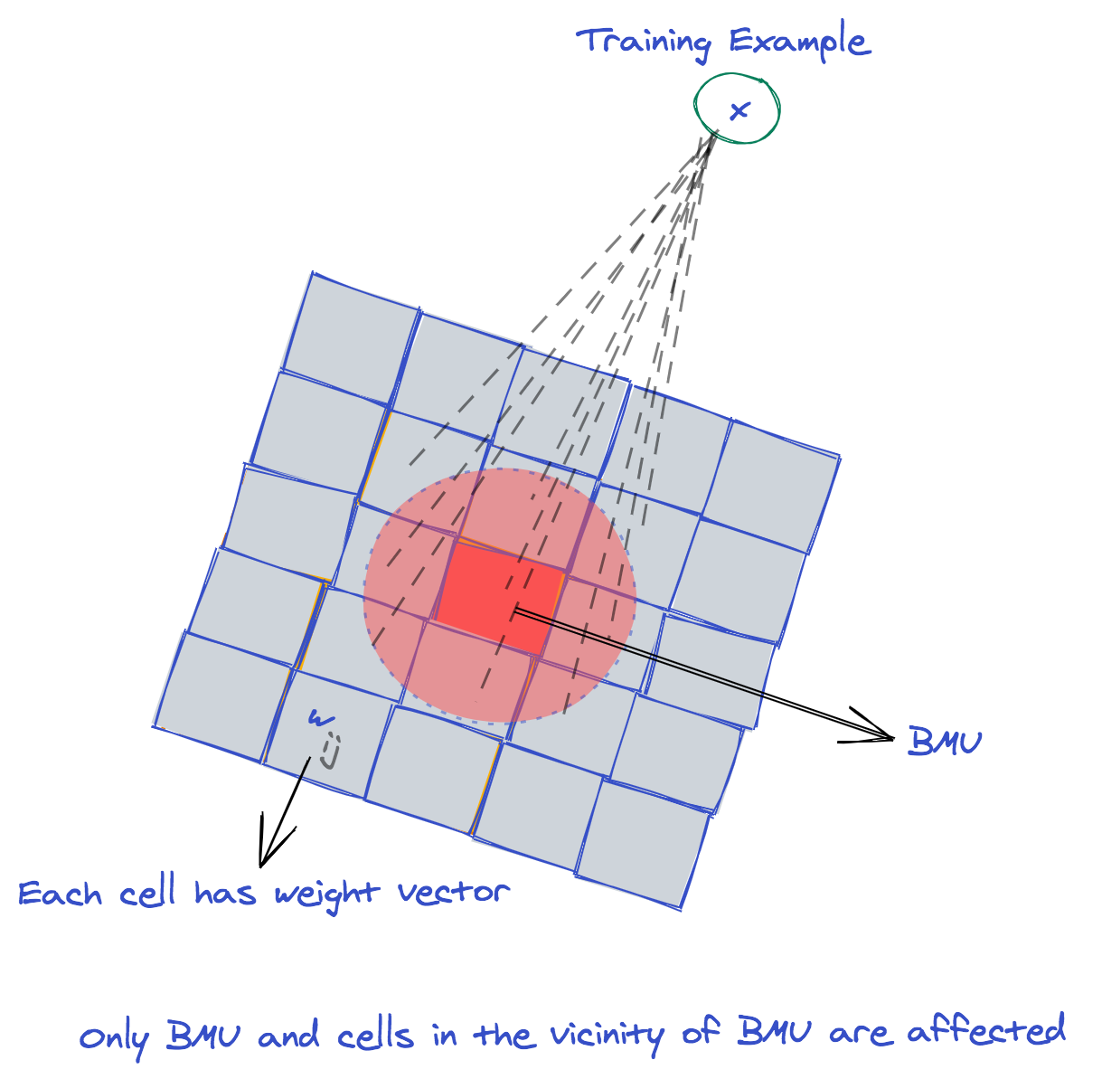
An SOM is trained using competitive learning.

Competitive Learning is a form of unsupervised learning, where constituent elements compete to produce a satisfying result, and only one gets to win the competition.

When a training example is input into the grid, the Best Matching Unit (BMU) is determined (competition winner). The BMU is the cell whose weights are closest to the training example.

Next, the BMU's weights and weights of the cells neighboring the BMU, are adapted to move closer to the input training instance. While there are other valid variants of training an SOM, we present the most popular and widely used implementation of the SOM in this guide.

As we'll be using some Python routines to demonstrate the functions used to train an SOM, let's import a few of the libraries we'll be using:

import numpy as np
import matplotlib.pyplot as plt

The Algorithm Behind Training Self-Organizing Maps

The basic algorithm for training an SOM is given below:

• Initialize all grid weights of the SOM

• Repeat until convergence or maximum epochs are reached

  • Shuffle the training examples

  • For each training instance xx

    • Find the best matching unit BMU

    • Update the weight vector of BMU and its neighboring cells

The three steps for initialization, finding the BMU, and updating the weights are explained in the following sections. Let's begin!

Initializing the SOM GRID

All the SOM grid weights can be initialized randomly. The SOM grid weights can also be initialized by randomly chosen examples from the training dataset.

Which one should you choose?

SOMs are sensitive to the initial weight of the map, so this choice affects the overall model. According to a case study performed by Ayodeji and Evgeny of University of Leicester and Siberian Federal University:

By comparing the proportion of final SOM map of RI (Random Initialization) which outperformed PCI (Principal Component Initialization) under the same conditions, it was observed that RI performed quite well for non-linear data sets.

However for quasi-linear datasets, the result remains inconclusive. In general, we can conclude that the hypothesis about advantages of the PCI is definitely wrong for essentially nonlinear datasets.

Random initialization outperforms non-random initialization for non-linear datasets. For quasi-linear datasets, it's not quite clear what approach wins consistently. Given these results - we'll stick to random initialization.

Finding the Best Matching Unit (BMU)

As mentioned earlier, the best matching unit is the cell of the SOM grid that is closest to the training example xx. One method of finding this unit is to compute the Euclidean distance of xx from the weight of each cell of the grid.

The cell with the minimum distance can be chosen as the BMU.

An important point to note is that Euclidean distance is not the only possible method of selecting the BMU. An alternative distance measure or a similarity metric can also be used to determine the BMU, and choosing this mainly depends on the data and model you're building specifically.

Updating the Weight Vector of BMU and Neighboring Cells

A training example xx effects various cells of the SOM grid by pulling the weights of these cells towards it. The maximum change occurs in the BMU and the influence of xx diminishes as we move away from the BMU in the SOM grid. For a cell with coordinates (i,j)(i,j), its weight wijwij is updated at epoch t+1t+1 as:

w(t+1)ij←w(t)ij+Δw(t)ijwij(t+1)←wij(t)+Δwij(t)

Where Δw(t)ijΔwij(t) is the change to be added to w(t)ijwij(t). It can be computed as:

Δw(t)ij=η(t)fi,j(g,h,σt)(x−w(t)ij)Δwij(t)=η(t)fi,j(g,h,σt)(x−wij(t))

For this expression:

• tt is the epoch number

• (g,h)(g,h) are the coordinates of BMU

• ηη is the learning rate

• σtσt is the radius

• fij(g,h,σt)fij(g,h,σt) is the neighborhood distance function

In the following sections, we'll present the details of this weight training expression.

The Learning Rate

The learning rate ηη is a constant in the range [0,1] and determines the step size of the weight vector towards the input training example. For η=0η=0, there is no change in the weight, and when η=1η=1 the weight vector wijwij take the value of xx.

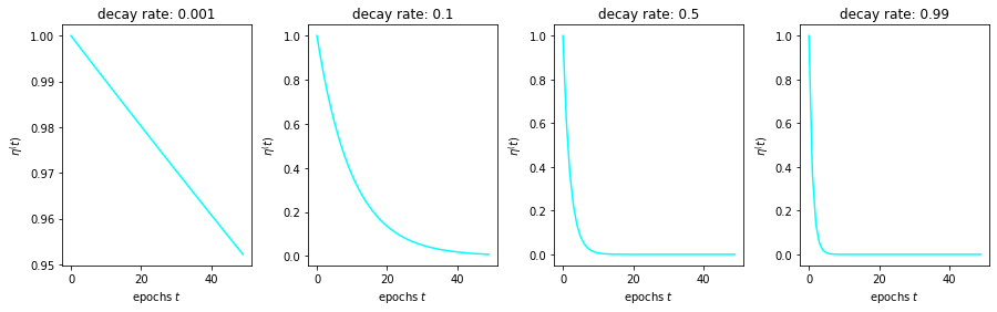
ηη is kept high at the start and decayed as the epochs proceed. One strategy for reducing the learning rate during the training phase is to use exponential decay:

η(t)=η0e−t∗λη(t)=η0e−t∗λ

Where λ<0λ<0 is the decay rate.

To understand how the learning rate changes with the decay rate, let's plot the learning rate against various epochs when the initial learning rate is set to one:

epochs = np.arange(0, 50)
lr_decay = [0.001, 0.1, 0.5, 0.99]
fig,ax = plt.subplots(nrows=1, ncols=4, figsize=(15,4))
plt_ind = np.arange(4) + 141
for decay, ind in zip(lr_decay, plt_ind):
    plt.subplot(ind)
    learn_rate = np.exp(-epochs * decay)
    plt.plot(epochs, learn_rate, c='cyan')
    plt.title('decay rate: ' + str(decay))
    plt.xlabel('epochs $t$')
    plt.ylabel('$\eta^(t)$')
fig.subplots_adjust(hspace=0.5, wspace=0.3)
plt.show()

learning rates for self organizing maps

The Neighborhood Distance Function

The neighborhood distance function is given by:

fij(g,h,σt)=e−d((i,j),(g,h))22σ2tfij(g,h,σt)=e−d((i,j),(g,h))22σt2

where d((i,j),(g,h))d((i,j),(g,h)) is the distance of coordinates (i,j)(i,j) of a cell from the BMU's coordinates (g,h)(g,h), and σtσt is the radius at epoch tt. Normally Euclidean distance is used to compute the distance, however, any other distance or similarity metric can be used.

As the distance of BMU with itself is zero, the weight change of the BMU reduces to:

Δwgh=η(x−wgh)Δwgh=η(x−wgh)

For a unit (i,j)(i,j) having a large distance from the BMU, the neighborhood distance function reduces to a near-zero value, leading to a very small magnitude of ΔwijΔwij. Hence, such units are unaffected by the training example xx. One training example, therefore, only affects the BMU and the cells in the close vicinity of the BMU. As we move away from the BMU the change in weights becomes less and less until it is negligible.

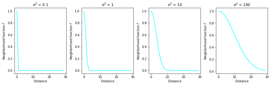
The radius determines the influence region of a training example xx. A high radius value affects a larger number of cells and a smaller radius affects only the BMU. A common strategy is to start with a large radius and reduce it as the epochs proceed, i.e.:

σt=σ0e−t∗βσt=σ0e−t∗β

Here β<0β<0 is the decay rate. The decay rate corresponding to radius has the same effect on the radius as the decay rate corresponding to the learning rate. To gain a deeper insight into the behavior of the neighborhood function, let's plot it against the distance for different values of the radius. A point to note in these graphs is that the distance function approaches a near-zero value as the distance exceeds 10 for σ2≤10σ2≤10.

We'll use this fact later to make training more efficient in the implementation part:

distance = np.arange(0, 30)
sigma_sq = [0.1, 1, 10, 100]
fig,ax = plt.subplots(nrows=1, ncols=4, figsize=(15,4))
plt_ind = np.arange(4) + 141
for s, ind in zip(sigma_sq, plt_ind):
    plt.subplot(ind)
    f = np.exp(-distance ** 2 / 2 / s)
    plt.plot(distance, f, c='cyan')
    plt.title('$\sigma^2$ = ' + str(s))
    plt.xlabel('Distance')
    plt.ylabel('Neighborhood function $f$')
fig.subplots_adjust(hspace=0.5, wspace=0.3)
plt.show()

decay rate for self organizing maps

Implementing a Self-Organizing Map in Python Using NumPy

As there is no built-in routine for an SOM in the de-facto standard machine learning library, Scikit-Learn, we'll do a quick implementation manually using NumPy. The unsupervised machine learning model is pretty straightforward and easy to implement.

We'll implement the SOM as a 2D mxn grid, hence requiring a 3D NumPy array. The third dimension is required for storing the weights in each cell:

# Return the (g,h) index of the BMU in the grid
def find_BMU(SOM,x):
    distSq = (np.square(SOM - x)).sum(axis=2)
    return np.unravel_index(np.argmin(distSq, axis=None), distSq.shape)
    
# Update the weights of the SOM cells when given a single training example
# and the model parameters along with BMU coordinates as a tuple
def update_weights(SOM, train_ex, learn_rate, radius_sq, 
                   BMU_coord, step=3):
    g, h = BMU_coord
    #if radius is close to zero then only BMU is changed
    if radius_sq < 1e-3:
        SOM[g,h,:] += learn_rate * (train_ex - SOM[g,h,:])
        return SOM
    # Change all cells in a small neighborhood of BMU
    for i in range(max(0, g-step), min(SOM.shape[0], g+step)):
        for j in range(max(0, h-step), min(SOM.shape[1], h+step)):
            dist_sq = np.square(i - g) + np.square(j - h)
            dist_func = np.exp(-dist_sq / 2 / radius_sq)
            SOM[i,j,:] += learn_rate * dist_func * (train_ex - SOM[i,j,:])   
    return SOM    

# Main routine for training an SOM. It requires an initialized SOM grid
# or a partially trained grid as parameter
def train_SOM(SOM, train_data, learn_rate = .1, radius_sq = 1, 
             lr_decay = .1, radius_decay = .1, epochs = 10):    
    learn_rate_0 = learn_rate
    radius_0 = radius_sq
    for epoch in np.arange(0, epochs):
        rand.shuffle(train_data)      
        for train_ex in train_data:
            g, h = find_BMU(SOM, train_ex)
            SOM = update_weights(SOM, train_ex, 
                                 learn_rate, radius_sq, (g,h))
        # Update learning rate and radius
        learn_rate = learn_rate_0 * np.exp(-epoch * lr_decay)
        radius_sq = radius_0 * np.exp(-epoch * radius_decay)            
    return SOM

Let's break down the key functions used to implement a Self-Organizing Map:

find_BMU() returns the grid cell coordinates of the best matching unit when given the SOM grid and a training example x. It computes the square of the Euclidean distance between each cell weight and x, and returns (g,h), i.e., the cell coordinates with the minimum distance.

The update_weights() function requires an SOM grid, a training example x, the parameters learn_rate and radius_sq, the coordinates of the best matching unit, and a step parameter. Theoretically, all cells of the SOM are updated on the next training example. However, we showed earlier that the change is negligible for cells that are far away from the BMU. Hence, we can make the code more efficient by changing only the cells in a small vicinity of the BMU. The step parameter specifies the maximum number of cells on the left, right, above, and below to change when updating the weights.

Finallt, the train_SOM() function implements the main training procedure of an SOM. It requires an initialized or partially trained SOM grid and train_data as parameters. The advantage is to be able to train the SOM from a previous trained stage. Additionally learn_rate and radius_sq parameters are required along with their corresponding decay rates lr_decay and radius_decay. The epochs parameter is set to 10 by default but can be changed if needed.

Running the Self-Organizing Map on a Practical Example

One of the commonly cited examples for training an SOM is that of random colors. We can train an SOM grid and easily visualize how various similar colors get arranged in neighboring cells.

Cells far away from each other have different colors.

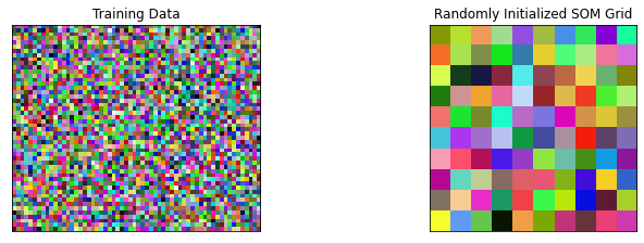
Let's run the train_SOM() function on a training data matrix filled with random RGB colors.

The code below initializes a training data matrix and an SOM grid with random RGB colors. It also displays the training data and the randomly initialized SOM grid. Note, the training matrix is a 3000x3 matrix, however, we have reshaped it to 50x60x3 matrix for visualization:

# Dimensions of the SOM grid
m = 10
n = 10
# Number of training examples
n_x = 3000
rand = np.random.RandomState(0)
# Initialize the training data
train_data = rand.randint(0, 255, (n_x, 3))
# Initialize the SOM randomly
SOM = rand.randint(0, 255, (m, n, 3)).astype(float)
# Display both the training matrix and the SOM grid
fig, ax = plt.subplots(
    nrows=1, ncols=2, figsize=(12, 3.5), 
    subplot_kw=dict(xticks=[], yticks=[]))
ax[0].imshow(train_data.reshape(50, 60, 3))
ax[0].title.set_text('Training Data')
ax[1].imshow(SOM.astype(int))
ax[1].title.set_text('Randomly Initialized SOM Grid')

randomly initialized self organizing map

Let's now train the SOM and check up on it every 5 epochs as a quick overview of its progress:

fig, ax = plt.subplots(
    nrows=1, ncols=4, figsize=(15, 3.5), 
    subplot_kw=dict(xticks=[], yticks=[]))
total_epochs = 0
for epochs, i in zip([1, 4, 5, 10], range(0,4)):
    total_epochs += epochs
    SOM = train_SOM(SOM, train_data, epochs=epochs)
    ax[i].imshow(SOM.astype(int))
    ax[i].title.set_text('Epochs = ' + str(total_epochs))

self organizing map training and results

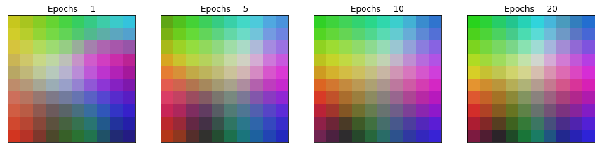
The example above is very interesting as it shows how the grid automatically arranges the RGB colors so that various shades of the same color are close together in the SOM grid. The arrangement takes place as early as the first epoch, but it's not ideal. We can see that the SOM converges in around 10 epochs and there are fewer changes in the subsequent epochs.

Effect of Learning Rate and Radius

To see how the learning rate varies for different learning rates and radii, we can run the SOM for 10 epochs when starting from the same initial grid. The code below trains the SOM for three different values of the learning rate and three different radii.

The SOM is rendered after 5 epochs for each simulation:

fig, ax = plt.subplots(
    nrows=3, ncols=3, figsize=(15, 15), 
    subplot_kw=dict(xticks=[], yticks=[]))

# Initialize the SOM randomly to the same state

for learn_rate, i in zip([0.001, 0.5, 0.99], [0, 1, 2]):
    for radius_sq, j in zip([0.01, 1, 10], [0, 1, 2]):
        rand = np.random.RandomState(0)
        SOM = rand.randint(0, 255, (m, n, 3)).astype(float)        
        SOM = train_SOM(SOM, train_data, epochs = 5,
                        learn_rate = learn_rate, 
                        radius_sq = radius_sq)
        ax[i][j].imshow(SOM.astype(int))
        ax[i][j].title.set_text('$\eta$ = ' + str(learn_rate) + 
                                ', $\sigma^2$ = ' + str(radius_sq))

effects and tuning self organizing map hyperparameters

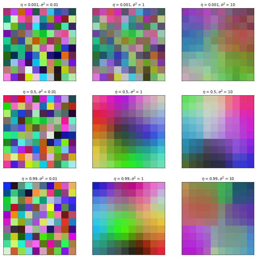
The example above shows that for radius values close to zero (first column), the SOM only changes the individual cells but not the neighboring cells. Hence, a proper map is not created regardless of the learning rate. A similar case is also encountered for smaller learning rates (first row, second column). As with any other machine learning algorithm, a good balance of parameters is required for ideal training.

Conclusions

In this guide, we discussed the theoretical model of an SOM and its detailed implementation. We demonstrated the SOM on RGB colors and showed how different shades of the same color organized themselves on a 2D grid.

While the SOMs are no longer very popular in the machine learning community, they remain a good model for data summary and visualization.